## Charts/Graphs: Neural Tangent Kernel Regime Performance
### Overview
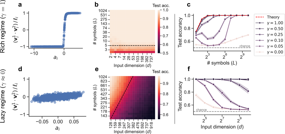
The image presents a series of six sub-plots (a-f) illustrating the relationship between input dimension (d), number of symbols (L), and test accuracy in two different neural network regimes: a "rich" regime (γ = 1) and a "lazy" regime (γ ≈ 0). The plots use scatter plots and heatmaps to visualize these relationships, with a theoretical curve provided for comparison.
### Components/Axes
* **Sub-plots a & d:** Scatter plots with `aᵢ` on the x-axis and `(v₁² - v₂²)/lᵢ` on the y-axis.
* Sub-plot a is labeled "Rich regime (γ = 1)".
* Sub-plot d is labeled "Lazy regime (γ ≈ 0)".
* **Sub-plots b & e:** Heatmaps showing "Test acc." (Test Accuracy) as a function of "Input dimension (d)" on the x-axis and "# symbols (L)" on the y-axis.
* Sub-plot b corresponds to the "Rich regime".
* Sub-plot e corresponds to the "Lazy regime".
* **Sub-plots c & f:** Line plots showing "Test accuracy" on the y-axis versus "# symbols (L)" on the x-axis (log scale).
* Sub-plot c corresponds to the "Rich regime".
* Sub-plot f corresponds to the "Lazy regime".
* **Legend (Sub-plot c):** Located in the top-right corner, the legend identifies different curves based on the value of γ (gamma):
* Red dashed line: "Theory"
* Black line with circles: γ = 0.00
* Dark grey line with squares: γ = 0.05
* Grey line with triangles pointing down: γ = 0.10
* Light grey line with diamonds: γ = 0.25
* Very light grey line with plus signs: γ = 0.50
* Dotted horizontal line: "chance"
* **Axis Scales:** The x and y axes use logarithmic scales in some plots (specifically, the number of symbols L in subplots c and f).
### Detailed Analysis or Content Details
**Sub-plot a (Rich Regime):**
The scatter plot shows a sharp transition in `(v₁² - v₂²)/lᵢ` around `aᵢ = 0`. For `aᵢ < 0`, the value is approximately -1. For `aᵢ > 0`, the value is approximately 1.
**Sub-plot b (Rich Regime Heatmap):**
The heatmap shows a strong positive correlation between input dimension (d) and test accuracy. As 'd' increases, the test accuracy increases, reaching a maximum value of approximately 1.0. The heatmap also shows that test accuracy increases with the number of symbols (L), but the effect is less pronounced than with the input dimension.
* Test accuracy ranges from approximately 0.5 to 1.0.
* Input dimension (d) ranges from 2 to 737.
* Number of symbols (L) ranges from 2 to 1024.
**Sub-plot c (Rich Regime Line Plots):**
The line plots show test accuracy as a function of the number of symbols (L).
* The "Theory" curve (red dashed) starts at a test accuracy of approximately 0.6 and rapidly increases to 1.0 as L increases.
* The γ = 0.00 curve (black circles) closely follows the "Theory" curve.
* As γ increases (0.05, 0.10, 0.25, 0.50), the curves shift downward, indicating lower test accuracy for a given number of symbols.
* The "chance" line is a horizontal line at approximately 0.6.
**Sub-plot d (Lazy Regime):**
The scatter plot shows a dense cluster of points around `(v₁² - v₂²)/lᵢ ≈ 0` for all values of `aᵢ` between approximately -0.05 and 0.05.
**Sub-plot e (Lazy Regime Heatmap):**
The heatmap shows a weaker correlation between input dimension (d) and test accuracy compared to the rich regime. Test accuracy increases slightly with increasing input dimension, but the increase is less dramatic. Test accuracy also increases with the number of symbols (L), but again, the effect is less pronounced.
* Test accuracy ranges from approximately 0.6 to 0.9.
* Input dimension (d) ranges from 159 to 918.
* Number of symbols (L) ranges from 128 to 1024.
**Sub-plot f (Lazy Regime Line Plots):**
The line plots show test accuracy as a function of the number of symbols (L).
* The γ = 0.00 curve (black circles) remains relatively flat, with test accuracy around 0.65-0.7 for all values of L.
* As γ increases (0.05, 0.10, 0.25, 0.50), the curves remain close to the "chance" level.
* The "Theory" curve is not present in this subplot.
### Key Observations
* The "rich" regime (γ = 1) exhibits a strong dependence of test accuracy on both input dimension and the number of symbols.
* The "lazy" regime (γ ≈ 0) shows a much weaker dependence on these parameters.
* The theoretical curve in the "rich" regime closely matches the experimental results for γ = 0.00.
* The "chance" level represents a baseline performance, and the curves for higher values of γ in the "rich" regime fall below this level.
* The scatter plots (a and d) visually represent the distribution of values in each regime, highlighting the distinct behavior.
### Interpretation
The data suggests a clear distinction in performance between the "rich" and "lazy" regimes of neural network training. In the "rich" regime, the network is able to learn complex representations, leading to high test accuracy as the input dimension and number of symbols increase. This behavior aligns with the theoretical predictions. In contrast, the "lazy" regime exhibits limited learning capacity, resulting in test accuracy that remains close to the "chance" level regardless of the input dimension or number of symbols. This indicates that the network is not effectively utilizing its parameters in this regime.
The difference in behavior can be attributed to the value of γ, which controls the learning rate and the degree of parameter updates during training. A higher value of γ (γ = 1) allows for more significant parameter changes, enabling the network to explore a wider range of representations. A lower value of γ (γ ≈ 0) restricts parameter updates, leading to a more conservative learning process and limited representational capacity.
The heatmaps and line plots provide a visual representation of these trends, allowing for a clear comparison of performance across different regimes and parameter settings. The outliers and anomalies, such as the downward shift in test accuracy for higher values of γ in the "rich" regime, highlight the importance of carefully tuning the learning rate to achieve optimal performance.