\n
## Diagram: LLM Development Pipeline for Math Problem Solving
### Overview
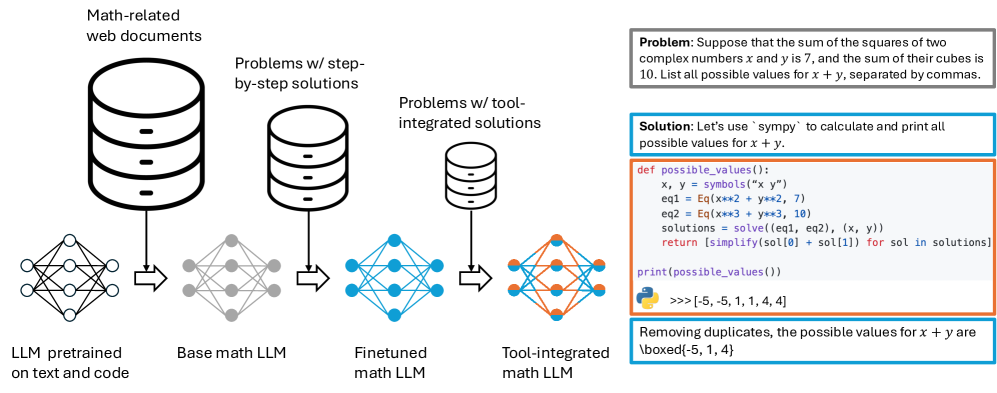
The image depicts a diagram illustrating a pipeline for developing Large Language Models (LLMs) specifically for solving math problems. The pipeline starts with a pre-trained LLM and progresses through stages of fine-tuning and tool integration, culminating in a tool-integrated math LLM. A sample math problem and its solution using Python code are presented on the right side of the diagram.
### Components/Axes
The diagram consists of four main stages, represented by cylindrical data stores and associated network graphs:
1. **LLM pretrained on text and code:** Represented by a cylinder labeled "LLM pretrained on text and code" and a network graph below it.
2. **Base math LLM:** Represented by a cylinder labeled "Base math LLM" and a network graph below it.
3. **Finetuned math LLM:** Represented by a cylinder labeled "Finetuned math LLM" and a network graph below it.
4. **Tool-integrated math LLM:** Represented by a cylinder labeled "Tool-integrated math LLM" and a network graph below it.
Arrows indicate the flow of development from one stage to the next.
On the right side, there is a text block containing a math problem and its solution. The problem is: "Suppose that the sum of the squares of two complex numbers x and y is 7, and the sum of their cubes is 10. List all possible values for x + y, separated by commas." The solution is provided in Python code using the 'sympy' library.
### Detailed Analysis or Content Details
The diagram shows a sequential process:
* **Stage 1:** An LLM is initially pre-trained on a broad dataset of text and code. The network graph below this stage appears relatively sparse.
* **Stage 2:** The pre-trained LLM is adapted into a "Base math LLM". The network graph below this stage shows increased connectivity.
* **Stage 3:** The base math LLM is further refined into a "Finetuned math LLM". The network graph below this stage shows even greater connectivity and complexity.
* **Stage 4:** Finally, the finetuned LLM is integrated with tools, resulting in a "Tool-integrated math LLM". The network graph below this stage is the most dense and complex.
The text block on the right provides a concrete example of the LLM's capabilities. The Python code defines a function `possible_values()` that uses `sympy` to solve the system of equations:
```python
x, y = symbols("x y")
eq1 = Eq(x**2 + y**2, 7)
eq2 = Eq(x**3 + y**3, 10)
solutions = solve((eq1, eq2), (x, y))
return [simplify(sol[0] + sol[1]) for sol in solutions]
print(possible_values())
>>> [-5, 1, 1, 4, 4]
```
The output of the code is `[-5, 1, 1, 4, 4]`. The text states that removing duplicates, the possible values for x + y are `[-5, 1, 4]`.
### Key Observations
The diagram highlights the iterative refinement process of LLM development. Each stage builds upon the previous one, increasing the model's specialization and capabilities. The increasing complexity of the network graphs suggests that the model learns more intricate relationships and patterns as it progresses through the pipeline. The example problem demonstrates the LLM's ability to solve mathematical problems using symbolic computation.
### Interpretation
The diagram illustrates a common approach to developing specialized LLMs. Starting with a general-purpose model and then fine-tuning it on a specific domain (in this case, mathematics) allows the model to leverage its existing knowledge while acquiring expertise in the target area. The integration of tools (like `sympy`) further enhances the model's capabilities by providing access to specialized algorithms and functions. The example problem and solution demonstrate the potential of this approach to automate complex mathematical reasoning. The pipeline suggests that the quality of the LLM's performance is directly related to the amount of fine-tuning and tool integration it receives. The network graphs visually represent the increasing complexity of the model's internal representation of mathematical concepts.