## Chart/Diagram Type: Spectral Region Analysis with 2-Norm Values
### Overview
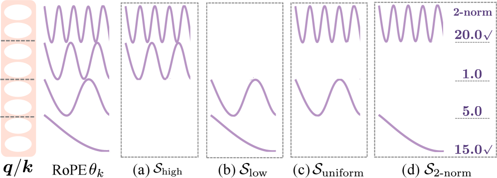
The image presents a technical diagram comparing spectral regions (S_high, S_low, S_uniform, S_2-norm) across different panels. A left panel shows "q/k" and "RoPE θ_k" with white circles, while the right side features a vertical axis labeled "2-norm" with values 20.0, 1.0, 5.0, and 15.0. Each panel (a-d) visualizes spectral oscillations and shaded regions, with varying complexity and 2-norm values.
### Components/Axes
- **Left Panel**:
- **X-axis**: "q/k" (horizontal axis).
- **Y-axis**: "RoPE θ_k" (vertical axis).
- **Visual Elements**: White circles stacked vertically, separated by dashed lines.
- **Right Side (Vertical Axis)**:
- **Label**: "2-norm" (vertical axis).
- **Values**: 20.0, 1.0, 5.0, 15.0 (listed in descending order from top to bottom).
- **Legend**: Purple lines (solid) and white shaded regions (dashed).
- **Panels (a-d)**:
- **(a) S_high**: High-frequency oscillations with multiple white shaded regions.
- **(b) S_low**: Lower-frequency oscillations with fewer shaded regions.
- **(c) S_uniform**: Minimal oscillations with uniform shading.
- **(d) S_2-norm**: Fewest oscillations and most uniform shading.
### Detailed Analysis
- **Panel (a) S_high**:
- **Oscillations**: 5–6 high-frequency waves.
- **Shaded Regions**: 3–4 white blocks (likely representing constraints or excluded ranges).
- **2-norm Value**: 20.0 (highest, top of the vertical axis).
- **Panel (b) S_low**:
- **Oscillations**: 2–3 lower-frequency waves.
- **Shaded Regions**: 2 white blocks.
- **2-norm Value**: 1.0 (lowest, bottom of the vertical axis).
- **Panel (c) S_uniform**:
- **Oscillations**: 1–2 waves.
- **Shaded Regions**: 1 large white block.
- **2-norm Value**: 5.0 (middle of the vertical axis).
- **Panel (d) S_2-norm**:
- **Oscillations**: 1 wave.
- **Shaded Regions**: 1 large white block.
- **2-norm Value**: 15.0 (second-highest, near the top).
### Key Observations
1. **Oscillation Complexity**: Decreases from (a) to (d), with S_high having the most oscillations and S_2-norm the fewest.
2. **Shaded Regions**: Increase in uniformity and coverage from (a) to (d), suggesting a trade-off between spectral complexity and normalization.
3. **2-norm Values**:
- S_high (20.0) and S_2-norm (15.0) have the highest values.
- S_low (1.0) and S_uniform (5.0) have significantly lower values, indicating potential anomalies or normalization effects.
4. **Vertical Axis Order**: The 2-norm values are listed as 20.0, 1.0, 5.0, 15.0, which may reflect a non-linear scaling or a labeling error.
### Interpretation
The diagram illustrates how spectral regions (S_high, S_low, S_uniform, S_2-norm) vary in complexity and 2-norm values. The reduction in oscillations and increase in uniform shading from (a) to (d) suggest a process of simplification or normalization. The 2-norm values (20.0, 1.0, 5.0, 15.0) may represent a metric (e.g., energy, error) that decreases with spectral complexity, though the irregular ordering of values (1.0 and 5.0) warrants further investigation. The white shaded regions likely denote excluded or constrained ranges, emphasizing the impact of spectral region selection on the analyzed metric.
### Notable Anomalies
- The 2-norm value for S_low (1.0) is significantly lower than S_uniform (5.0), despite S_low having fewer oscillations. This could indicate a non-linear relationship between spectral complexity and the 2-norm metric.
- The vertical axis labels (20.0, 1.0, 5.0, 15.0) are not in descending order, suggesting a possible error in the diagram or a specific scaling rationale.
### Conclusion
This diagram highlights the interplay between spectral region characteristics (frequency, shading) and a normalized metric (2-norm). The trends suggest that higher-frequency regions (S_high) are more complex and have higher 2-norm values, while lower-frequency regions (S_2-norm) are simpler but exhibit intermediate 2-norm values. Further analysis is needed to resolve the anomalies in the 2-norm scaling.