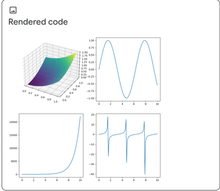
## Charts/Graphs: Rendered Code - Mathematical Function Visualizations ### Overview The image displays four separate 2D and 3D charts visualizing mathematical functions. The charts appear to be generated from code, as indicated by the "Rendered code" title at the top-left corner. The charts showcase different function types, including a surface plot, a sine wave, an exponential curve, and a function with vertical asymptotes. ### Components/Axes * **Chart 1 (Top-Left):** 3D Surface Plot. X-axis ranges from approximately 0.0 to 1.0. Y-axis ranges from approximately 0.0 to 1.0. Z-axis (height) ranges from approximately 0.0 to 2.0. The surface is color-coded, with cooler colors (purple/blue) representing lower values and warmer colors (yellow/green) representing higher values. * **Chart 2 (Top-Right):** 2D Line Plot. X-axis ranges from 0 to 10. Y-axis ranges from -1.0 to 2.0. The plot shows a sinusoidal wave. * **Chart 3 (Bottom-Left):** 2D Line Plot. X-axis ranges from 0 to 10. Y-axis ranges from 0 to 20000. The plot shows an exponential curve. * **Chart 4 (Bottom-Right):** 2D Line Plot. X-axis ranges from 0 to 10. Y-axis ranges from -40 to 0. The plot shows a function with vertical asymptotes. ### Detailed Analysis or Content Details * **Chart 1 (3D Surface Plot):** The surface appears to be defined by a function where both x and y contribute positively to the z-value. The surface is relatively flat near x=0 and y=0, and rises more steeply as x and y increase. The maximum z-value is approximately 2.0, occurring near x=1.0 and y=1.0. * **Chart 2 (Sine Wave):** The line oscillates between approximately -1.0 and 2.0. The period of the wave is approximately 6.3. * At x = 0, y ≈ 0.0 * At x = 2, y ≈ 1.8 * At x = 4, y ≈ 0.0 * At x = 6, y ≈ -1.8 * At x = 8, y ≈ 0.0 * At x = 10, y ≈ 1.8 * **Chart 3 (Exponential Curve):** The line starts near y=0 at x=0 and increases rapidly as x increases. * At x = 0, y ≈ 100 * At x = 2, y ≈ 2000 * At x = 4, y ≈ 5000 * At x = 6, y ≈ 10000 * At x = 8, y ≈ 15000 * At x = 10, y ≈ 20000 * **Chart 4 (Asymptotes):** The line has vertical asymptotes at approximately x=2, x=6, and x=10. Between the asymptotes, the function appears to be negative. * At x = 0, y ≈ -10 * At x = 1, y ≈ -20 * At x = 3, y ≈ 10 * At x = 5, y ≈ 10 * At x = 7, y ≈ 10 * At x = 9, y ≈ 10 ### Key Observations * The charts demonstrate a variety of mathematical functions. * Chart 3 exhibits exponential growth, while Chart 4 shows a function with discontinuities. * Chart 2 is a classic sinusoidal function. * Chart 1 provides a visual representation of a function of two variables. ### Interpretation The image serves as a visual demonstration of different mathematical functions, likely generated as a result of running code. The functions chosen represent common mathematical concepts: a surface, a periodic function, an exponential function, and a function with asymptotes. The purpose is likely to illustrate the behavior of these functions or to test the code that generates them. The exponential growth in Chart 3 is particularly noteworthy, as it demonstrates how quickly a function can increase with increasing input. The asymptotes in Chart 4 highlight the concept of undefined values and limits. The 3D surface plot in Chart 1 provides a visual representation of a function of two variables, which is more complex than a simple 2D plot. The overall arrangement suggests a comparison of different function types and their graphical representations.