## Line Graph: Probability Distribution P(q) at T = 0.31, Instance 1
### Overview
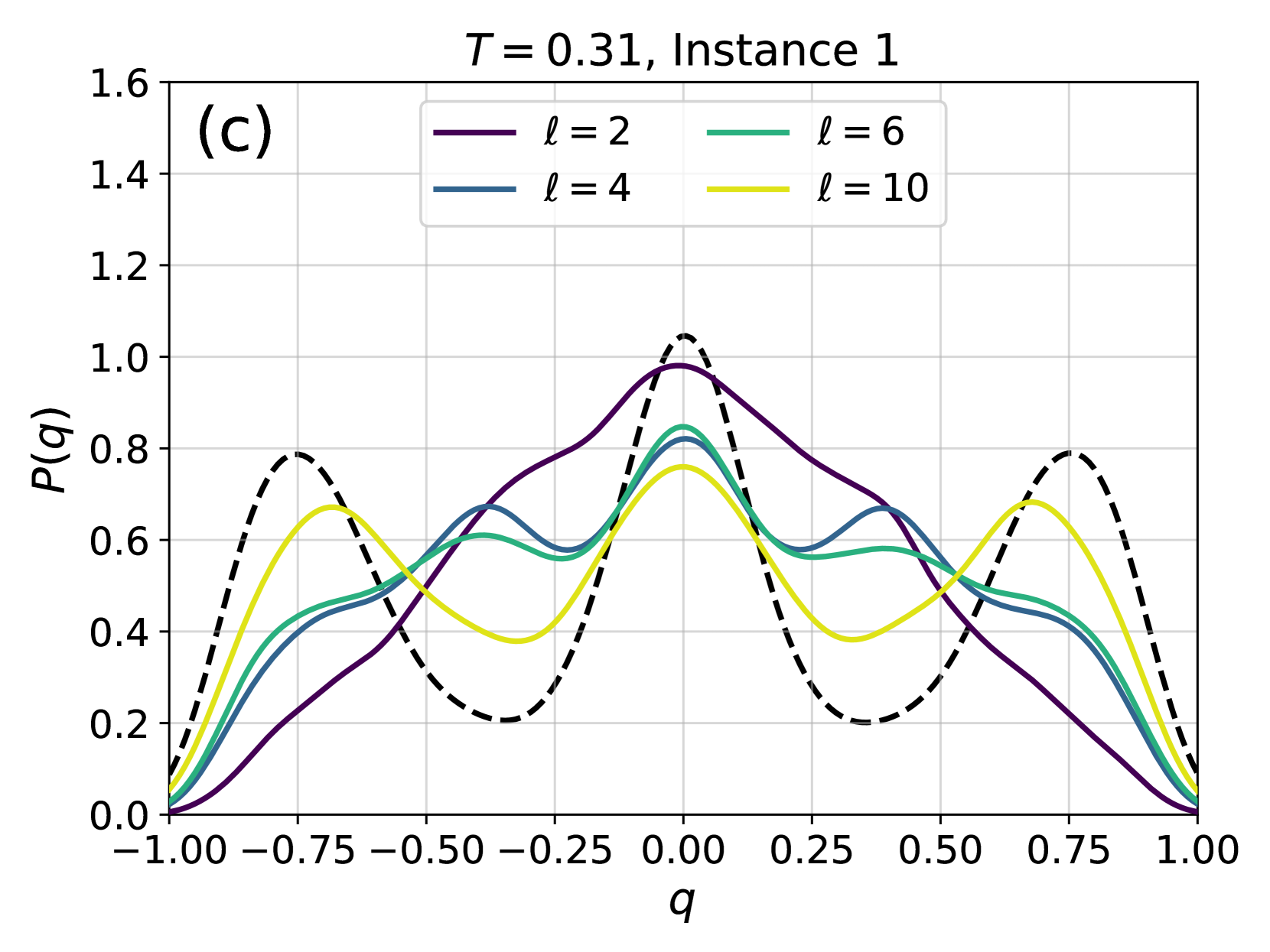
The graph displays probability distributions P(q) as a function of q for four distinct values of ℓ (2, 4, 6, 10) at a fixed temperature T = 0.31. A dashed reference line is included for comparison. All distributions are symmetric about q = 0, with peaks centered at q = 0 and secondary peaks at q ≈ ±0.75.
### Components/Axes
- **X-axis (q)**: Ranges from -1.00 to 1.00 in increments of 0.25.
- **Y-axis (P(q))**: Ranges from 0.0 to 1.6 in increments of 0.2.
- **Legend**: Located in the top-right corner, mapping colors to ℓ values:
- Purple: ℓ = 2
- Teal: ℓ = 6
- Blue: ℓ = 4
- Yellow: ℓ = 10
- **Dashed Line**: Black dashed curve, likely a reference distribution.
### Detailed Analysis
1. **ℓ = 2 (Purple Line)**:
- Sharpest peak at q = 0 (P(q) ≈ 1.0).
- Secondary peaks at q ≈ ±0.75 (P(q) ≈ 0.8).
- Narrowest distribution overall.
2. **ℓ = 4 (Blue Line)**:
- Peak at q = 0 (P(q) ≈ 0.9).
- Secondary peaks at q ≈ ±0.75 (P(q) ≈ 0.7).
- Broader than ℓ = 2 but narrower than ℓ = 6/10.
3. **ℓ = 6 (Teal Line)**:
- Peak at q = 0 (P(q) ≈ 0.85).
- Secondary peaks at q ≈ ±0.75 (P(q) ≈ 0.6).
- Broader than ℓ = 4, with reduced peak height.
4. **ℓ = 10 (Yellow Line)**:
- Peak at q = 0 (P(q) ≈ 0.8).
- Secondary peaks at q ≈ ±0.75 (P(q) ≈ 0.5).
- Broadest distribution, lowest peak height.
5. **Dashed Line**:
- Peaks at q ≈ ±0.75 (P(q) ≈ 1.0).
- Flat minimum at q = 0 (P(q) ≈ 0.4).
- Symmetric but inverted relative to solid lines.
### Key Observations
- **Inverse Relationship**: Higher ℓ values correlate with broader distributions and lower peak probabilities at q = 0.
- **Secondary Peaks**: All solid lines exhibit secondary maxima at q ≈ ±0.75, matching the dashed line's primary peaks.
- **Dashed Line Contrast**: The dashed line’s inverted profile suggests it represents a complementary or orthogonal distribution (e.g., q²-dependent terms).
### Interpretation
The data suggests that ℓ modulates the width and height of the probability distribution P(q). Lower ℓ values (e.g., ℓ = 2) produce sharper, more localized distributions, while higher ℓ values (e.g., ℓ = 10) yield broader, flatter distributions. The dashed line’s secondary peaks at q ≈ ±0.75 may represent boundary effects or interactions between system components. The temperature T = 0.31 likely stabilizes the system in a regime where these distributions are thermally equilibrated. The inverse scaling of peak height with ℓ implies that larger ℓ values suppress central concentration in favor of distributed states.