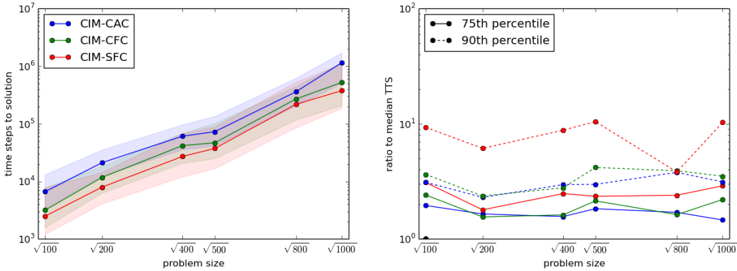
## Combined Line Chart: Algorithm Performance vs. Problem Size ### Overview The image presents two line charts side-by-side, comparing the performance of different algorithms (CIM-CAC, CIM-CFC, CIM-SFC) against varying problem sizes. The left chart displays "time steps to solution" on a logarithmic scale, while the right chart shows the "ratio to median TTS" (Time To Solution), also on a logarithmic scale. The x-axis for both charts represents "problem size," expressed as the square root of the actual problem size. ### Components/Axes **Left Chart:** * **Title:** time steps to solution * **Y-axis:** time steps to solution (logarithmic scale) * Axis markers: 10^3, 10^4, 10^5, 10^6, 10^7 * **X-axis:** problem size (square root) * Axis markers: √100, √200, √400, √500, √800, √1000 * **Legend (top-left):** * Blue: CIM-CAC * Green: CIM-CFC * Red: CIM-SFC * Shaded regions around each line represent some measure of variance or uncertainty. **Right Chart:** * **Title:** ratio to median TTS * **Y-axis:** ratio to median TTS (logarithmic scale) * Axis markers: 10^0, 10^1, 10^2 * **X-axis:** problem size (square root) * Axis markers: √100, √200, √400, √500, √800, √1000 * **Legend (top-left):** * Black (solid line): 75th percentile * Black (dashed line): 90th percentile ### Detailed Analysis **Left Chart (Time Steps to Solution):** * **CIM-CAC (Blue):** The line slopes upward, indicating that the time steps to solution increase with problem size. * √100: ~3000 * √200: ~20000 * √400: ~45000 * √500: ~60000 * √800: ~200000 * √1000: ~400000 * **CIM-CFC (Green):** The line slopes upward, indicating that the time steps to solution increase with problem size. * √100: ~2500 * √200: ~10000 * √400: ~30000 * √500: ~40000 * √800: ~100000 * √1000: ~250000 * **CIM-SFC (Red):** The line slopes upward, indicating that the time steps to solution increase with problem size. * √100: ~2000 * √200: ~8000 * √400: ~25000 * √500: ~35000 * √800: ~80000 * √1000: ~200000 **Right Chart (Ratio to Median TTS):** * **75th percentile (Black, solid):** The line is relatively flat, suggesting the 75th percentile ratio to median TTS remains relatively constant across problem sizes. * √100: ~1 * √200: ~1.5 * √400: ~1.5 * √500: ~1.3 * √800: ~1.5 * √1000: ~1.5 * **90th percentile (Black, dashed):** The line fluctuates more than the 75th percentile, but generally stays within a small range. * √100: ~2.5 * √200: ~2 * √400: ~2.5 * √500: ~3 * √800: ~2 * √1000: ~2.5 ### Key Observations * In the left chart, all three algorithms (CIM-CAC, CIM-CFC, CIM-SFC) exhibit an increase in "time steps to solution" as the problem size increases. * CIM-CAC consistently requires more time steps to solution than CIM-CFC and CIM-SFC. * In the right chart, the 75th and 90th percentile ratios to median TTS are relatively stable across different problem sizes. * The ratio to median TTS for CIM-SFC is higher than CIM-CAC and CIM-CFC at smaller problem sizes, but converges as the problem size increases. ### Interpretation The left chart demonstrates the expected behavior that larger problems require more computational steps to solve. The relative positioning of the lines suggests that CIM-CAC is generally less efficient in terms of time steps than CIM-CFC and CIM-SFC for the problem set being analyzed. The right chart provides insight into the variability of the algorithms' performance. The relatively stable 75th and 90th percentile lines indicate that the distribution of Time To Solution (TTS) is consistent across different problem sizes. The higher ratio to median TTS for CIM-SFC at smaller problem sizes suggests that it may have more variable performance in those scenarios, potentially due to factors like initialization or search space exploration. As the problem size increases, the algorithms' performance becomes more consistent relative to their median TTS.