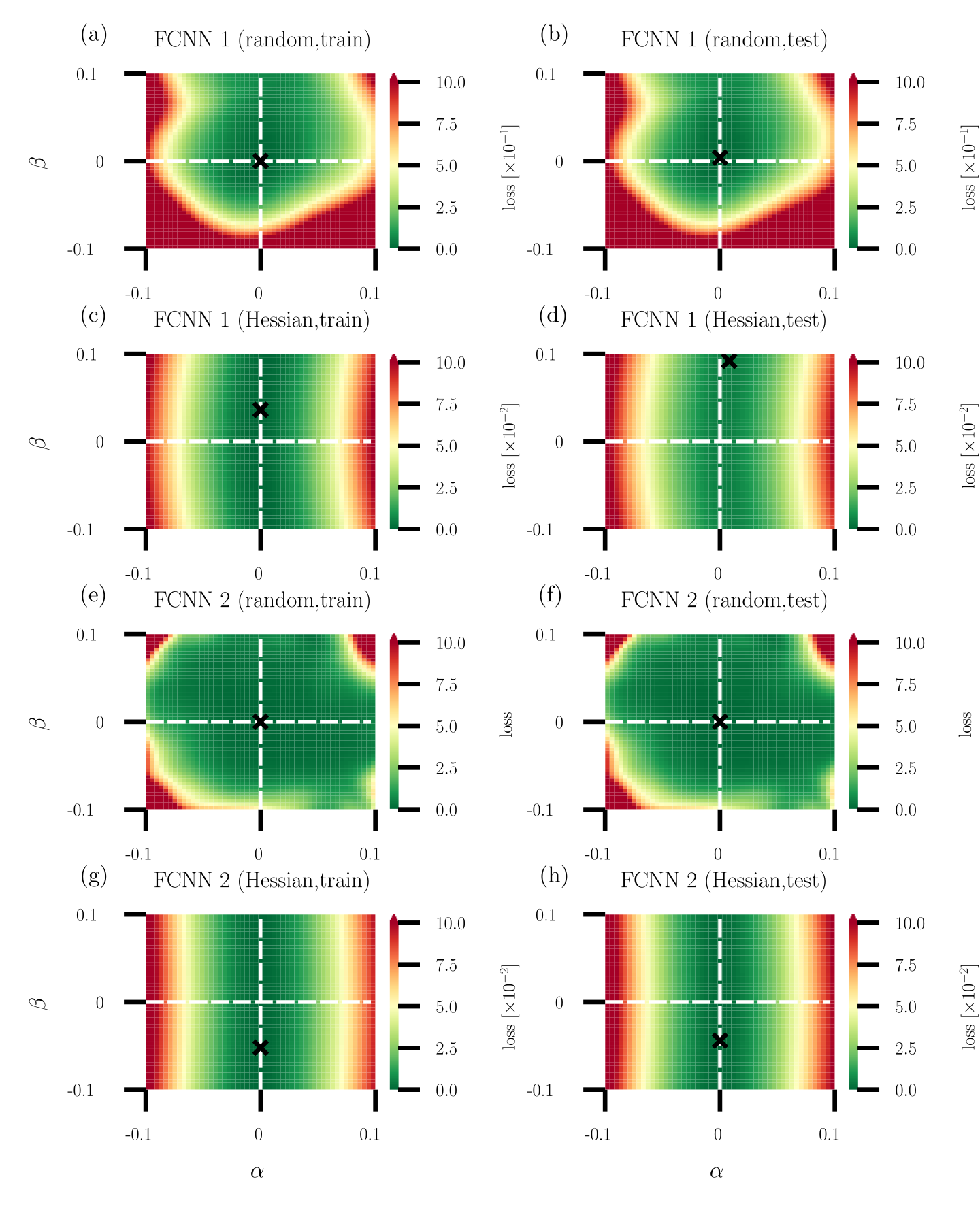
## Heatmap: Loss Landscapes of FCNN Models ### Overview The image presents a series of heatmaps visualizing the loss landscapes of Fully Connected Neural Networks (FCNNs) under different training conditions and architectures. Each heatmap represents the loss value as a function of two parameters, alpha (α) and beta (β). The heatmaps are arranged in a 2x4 grid, varying by network architecture (FCNN 1 vs. FCNN 2), training method (random vs. Hessian), and dataset (train vs. test). ### Components/Axes * **X-axis (Horizontal):** α (alpha), ranging from -0.1 to 0.1. * **Y-axis (Vertical):** β (beta), ranging from -0.1 to 0.1. * **Color Scale (Right):** Represents the loss value. The scale ranges from 0.0 to 10.0, with color transitions indicating different loss levels. Red indicates higher loss, and green indicates lower loss. The loss is scaled by 10^-1 for the top row and 10^-2 for the remaining rows. * **Titles:** Each subplot has a title indicating the FCNN architecture (1 or 2), training method (random or Hessian), and dataset (train or test). * (a) FCNN 1 (random, train) * (b) FCNN 1 (random, test) * (c) FCNN 1 (Hessian, train) * (d) FCNN 1 (Hessian, test) * (e) FCNN 2 (random, train) * (f) FCNN 2 (random, test) * (g) FCNN 2 (Hessian, train) * (h) FCNN 2 (Hessian, test) * **Axes Markers:** The axes are marked at -0.1, 0, and 0.1 for both α and β. * **Crosshair:** Each plot contains a dashed white crosshair centered at (0,0). A black 'X' is located at the intersection of the crosshair. ### Detailed Analysis **Subplot (a): FCNN 1 (random, train)** * Trend: A green (low loss) region is centered around (0,0), surrounded by a red (high loss) region in the corners. * Loss values: The minimum loss (green) is approximately 0 near the center. The maximum loss (red) reaches approximately 10 * 10^-1 = 1.0 in the corners. **Subplot (b): FCNN 1 (random, test)** * Trend: Similar to (a), a green (low loss) region is centered around (0,0), surrounded by a red (high loss) region in the corners. * Loss values: The minimum loss (green) is approximately 0 near the center. The maximum loss (red) reaches approximately 10 * 10^-1 = 1.0 in the corners. **Subplot (c): FCNN 1 (Hessian, train)** * Trend: A horizontal green band (low loss) is centered around β = 0, with red regions (high loss) above and below. * Loss values: The minimum loss (green) is approximately 0 along the horizontal band. The maximum loss (red) reaches approximately 10 * 10^-2 = 0.1 at the top and bottom edges. **Subplot (d): FCNN 1 (Hessian, test)** * Trend: Similar to (c), a horizontal green band (low loss) is centered around β = 0, with red regions (high loss) above and below. * Loss values: The minimum loss (green) is approximately 0 along the horizontal band. The maximum loss (red) reaches approximately 10 * 10^-2 = 0.1 at the top and bottom edges. **Subplot (e): FCNN 2 (random, train)** * Trend: A green (low loss) region is centered around (0,0), with red regions (high loss) in the corners. The green region appears slightly more elongated vertically compared to FCNN 1. * Loss values: The minimum loss (green) is approximately 0 near the center. The maximum loss (red) reaches approximately 10 * 10^-2 = 0.1 in the corners. **Subplot (f): FCNN 2 (random, test)** * Trend: Similar to (e), a green (low loss) region is centered around (0,0), with red regions (high loss) in the corners. * Loss values: The minimum loss (green) is approximately 0 near the center. The maximum loss (red) reaches approximately 10 * 10^-2 = 0.1 in the corners. **Subplot (g): FCNN 2 (Hessian, train)** * Trend: A horizontal green band (low loss) is centered around β = 0, with red regions (high loss) above and below. * Loss values: The minimum loss (green) is approximately 0 along the horizontal band. The maximum loss (red) reaches approximately 10 * 10^-2 = 0.1 at the top and bottom edges. **Subplot (h): FCNN 2 (Hessian, test)** * Trend: Similar to (g), a horizontal green band (low loss) is centered around β = 0, with red regions (high loss) above and below. * Loss values: The minimum loss (green) is approximately 0 along the horizontal band. The maximum loss (red) reaches approximately 10 * 10^-2 = 0.1 at the top and bottom edges. ### Key Observations * **Training Method Impact:** The Hessian training method results in a loss landscape with a clear horizontal band of low loss around β = 0 for both FCNN 1 and FCNN 2. The random training method results in a more localized low-loss region around (0,0). * **Network Architecture Impact:** The loss landscapes for FCNN 1 and FCNN 2 are qualitatively similar for both random and Hessian training methods. However, the scale of the loss differs, with FCNN 1 (random) having a higher loss scale (10^-1) compared to the others (10^-2). * **Train vs. Test:** The loss landscapes for train and test datasets are very similar for each combination of network architecture and training method, suggesting good generalization. ### Interpretation The heatmaps visualize how the loss function changes as the parameters α and β are varied. The goal is to find the values of α and β that minimize the loss, represented by the green regions. The Hessian training method appears to create a loss landscape where the loss is less sensitive to changes in α, as indicated by the horizontal bands of low loss. This might suggest that the Hessian method leads to a more robust solution with respect to variations in α. The random training method, on the other hand, results in a more localized minimum around (0,0), suggesting that the solution is more sensitive to changes in both α and β. The similarity between the train and test loss landscapes indicates that the models are generalizing well to unseen data. The difference in loss scale between FCNN 1 (random) and the other configurations suggests that FCNN 1 (random) might be less efficient or require further optimization.

\n ## Heatmaps: FCNN Parameter Space Loss Visualization ### Overview The image presents eight heatmaps, each visualizing the loss function of a Fully Connected Neural Network (FCNN) across a parameter space defined by α and β. Each heatmap corresponds to a specific training/testing scenario and network configuration (FCNN 1 or FCNN 2, trained with either random or Hessian initialization). A black 'x' marks the point of minimum loss on each heatmap. The color scale represents the loss value, ranging from 0.0 to 10.0. ### Components/Axes Each heatmap shares the following components: * **X-axis:** Labeled "α" with a scale ranging from -0.1 to 0.1. * **Y-axis:** Labeled "β" with a scale ranging from -0.1 to 0.1. * **Colorbar:** Located to the right of each heatmap, representing the "Loss [x10⁻²]" scale from 0.0 (dark green) to 10.0 (dark red). * **Title:** Each heatmap has a title indicating the network (FCNN 1 or FCNN 2) and the training method (random or Hessian) along with whether it represents the training or testing set. * **Minimum Loss Marker:** A black 'x' indicates the approximate location of the minimum loss within the parameter space. ### Detailed Analysis or Content Details Here's a breakdown of each heatmap, including approximate coordinates of the minimum loss marker ('x'): **(a) FCNN 1 (random, train):** * Trend: The loss appears to decrease towards the center of the parameter space. * Minimum Loss Location: Approximately (0.0, 0.0). * Loss Value at Minimum: Approximately 0.5 (estimated from the colorbar). **(b) FCNN 1 (random, test):** * Trend: Similar to (a), loss decreases towards the center. * Minimum Loss Location: Approximately (0.0, 0.0). * Loss Value at Minimum: Approximately 1.0 (estimated from the colorbar). **(c) FCNN 1 (Hessian, train):** * Trend: Loss is concentrated around the center, with a clear minimum. * Minimum Loss Location: Approximately (0.0, 0.0). * Loss Value at Minimum: Approximately 0.1 (estimated from the colorbar). **(d) FCNN 1 (Hessian, test):** * Trend: Similar to (c), loss is concentrated around the center. * Minimum Loss Location: Approximately (0.0, 0.0). * Loss Value at Minimum: Approximately 0.5 (estimated from the colorbar). **(e) FCNN 2 (random, train):** * Trend: Loss is more spread out, with a broad minimum. * Minimum Loss Location: Approximately (0.0, 0.0). * Loss Value at Minimum: Approximately 1.5 (estimated from the colorbar). **(f) FCNN 2 (random, test):** * Trend: Similar to (e), loss is spread out. * Minimum Loss Location: Approximately (0.0, 0.0). * Loss Value at Minimum: Approximately 2.0 (estimated from the colorbar). **(g) FCNN 2 (Hessian, train):** * Trend: Loss is concentrated around the center, with a clear minimum. * Minimum Loss Location: Approximately (0.0, 0.0). * Loss Value at Minimum: Approximately 0.2 (estimated from the colorbar). **(h) FCNN 2 (Hessian, test):** * Trend: Similar to (g), loss is concentrated around the center. * Minimum Loss Location: Approximately (0.0, 0.0). * Loss Value at Minimum: Approximately 0.7 (estimated from the colorbar). ### Key Observations * **Hessian Initialization:** Using the Hessian initialization consistently results in lower loss values, both during training and testing, compared to random initialization for both FCNNs. * **FCNN 1 vs. FCNN 2:** FCNN 1 generally achieves lower loss values than FCNN 2, particularly when using Hessian initialization. * **Training vs. Testing:** Loss values are generally higher on the test set than on the training set for both networks and both initialization methods, indicating some degree of overfitting. * **Minimum Location:** The minimum loss consistently occurs around α = 0.0 and β = 0.0 for all scenarios. ### Interpretation The heatmaps demonstrate the impact of initialization methods (random vs. Hessian) on the training and generalization performance of two different FCNN architectures. The Hessian initialization appears to be a more effective strategy for finding parameter values that minimize loss, leading to better performance on both training and testing data. The consistent location of the minimum loss at α = 0.0 and β = 0.0 suggests that these parameter values represent a stable and optimal configuration for both networks. The difference in loss values between FCNN 1 and FCNN 2 indicates that the network architecture itself plays a significant role in determining the model's ability to learn and generalize. The higher loss on the test set compared to the training set suggests that both networks are prone to overfitting, and regularization techniques might be necessary to improve their generalization performance. The visualization provides a clear and intuitive way to understand the relationship between network parameters and loss, aiding in the optimization and design of FCNNs.

## Heatmap Grid: Loss Landscapes for Fully Connected Neural Networks (FCNNs) ### Overview The image displays a 4x2 grid of eight heatmap plots, labeled (a) through (h). Each plot visualizes the loss landscape of a Fully Connected Neural Network (FCNN) in a 2D parameter subspace defined by axes `α` and `β`. The plots compare two different network architectures (FCNN 1 and FCNN 2), two parameter initialization methods ("random" and "Hessian"), and two dataset splits ("train" and "test"). The color intensity represents the loss value at each coordinate pair (α, β). ### Components/Axes * **Grid Structure:** 4 rows x 2 columns. * **Subplot Labels:** (a), (b), (c), (d), (e), (f), (g), (h) in the top-left corner of each plot. * **Subplot Titles:** Each title follows the format: `[Model] ([Initialization], [Dataset])`. * (a) FCNN 1 (random,train) * (b) FCNN 1 (random,test) * (c) FCNN 1 (Hessian,train) * (d) FCNN 1 (Hessian,test) * (e) FCNN 2 (random,train) * (f) FCNN 2 (random,test) * (g) FCNN 2 (Hessian,train) * (h) FCNN 2 (Hessian,test) * **Axes:** * **X-axis (Horizontal):** Labeled `α` at the bottom of the grid (plots g, h). Range: -0.1 to 0.1. Major ticks at -0.1, 0, 0.1. * **Y-axis (Vertical):** Labeled `β` on the left side of the grid (plots a, c, e, g). Range: -0.1 to 0.1. Major ticks at -0.1, 0, 0.1. * **Color Bar (Legend):** Located to the right of each heatmap. It maps color to loss value. * **Color Scale:** A gradient from dark green (low loss) through yellow to dark red (high loss). * **Labels & Scale:** * Plots (a), (b), (e), (f) [Random Init]: Labeled `loss [×10⁻¹]`. Scale ranges from 0.0 to 10.0. This indicates the displayed values should be multiplied by 0.1 (e.g., 10.0 represents a loss of 1.0). * Plots (c), (d) [FCNN 1, Hessian Init]: Labeled `loss [×10⁻²]`. Scale ranges from 0.0 to 10.0. This indicates the displayed values should be multiplied by 0.01 (e.g., 10.0 represents a loss of 0.1). * Plots (g), (h) [FCNN 2, Hessian Init]: Labeled `loss`. Scale ranges from 0.0 to 10.0. No multiplier is indicated, suggesting the values are as displayed. * **Reference Lines:** White dashed lines cross at (α=0, β=0) in each plot. * **Marked Point:** A black 'x' marks a specific point in each landscape, likely the converged solution or minimum found during training. ### Detailed Analysis **1. Random Initialization Landscapes (Plots a, b, e, f):** * **Trend/Shape:** The low-loss region (green) forms a broad, roughly circular or elliptical basin centered near (0,0). Loss increases radially outward, transitioning to yellow and then red at the edges of the [-0.1, 0.1] domain. * **Marked Point ('x'):** Located precisely at the intersection of the white dashed lines, (α=0, β=0), in all four random initialization plots. * **Loss Scale:** The color bar multiplier of `×10⁻¹` indicates the loss values in these landscapes are an order of magnitude larger than those in the Hessian-initialized FCNN 1 plots. * **Train vs. Test:** The landscapes for train (a, e) and test (b, f) are visually very similar for each respective model, suggesting the loss surface geometry generalizes well. **2. Hessian Initialization Landscapes (Plots c, d, g, h):** * **Trend/Shape:** The landscapes are dominated by vertical bands. The lowest loss (green) forms a vertical stripe centered around α=0. Loss increases as |α| increases, moving into yellow and red regions on the left and right sides. The variation along the β-axis is much less pronounced compared to the α-axis. * **Marked Point ('x') Position:** * **FCNN 1 (c, d):** The 'x' is offset from the center. In (c) train, it is at approximately (α=0, β≈0.03). In (d) test, it is at approximately (α=0, β≈0.09). * **FCNN 2 (g, h):** The 'x' is offset in the negative β direction. In both (g) train and (h) test, it is at approximately (α=0, β≈-0.03). * **Loss Scale:** * FCNN 1 (c, d): The `×10⁻²` multiplier indicates these loss values are 100 times smaller than those in the random initialization plots for FCNN 1. * FCNN 2 (g, h): The scale has no multiplier, suggesting loss values are directly comparable to the 0-10 range, but the landscape shape is fundamentally different from its random initialization counterpart. ### Key Observations 1. **Dramatic Landscape Change with Initialization:** The most striking feature is the complete transformation of the loss landscape geometry when switching from random to Hessian-based initialization. Random init yields isotropic (circular) basins, while Hessian init creates anisotropic (vertically elongated) valleys. 2. **Consistency Across Train/Test:** For a given model and initialization, the train and test loss landscapes are remarkably similar in shape and scale. This implies the local geometry of the loss surface around the solution is determined more by the model and initialization than by the specific data split. 3. **Divergent Convergence Points:** The black 'x' marks show that Hessian initialization leads the optimization to converge to different points in the (α, β) subspace compared to random initialization (which always finds (0,0)). Furthermore, the converged point differs between FCNN 1 and FCNN 2 under Hessian init. 4. **Scale of Loss:** The loss values at the minima (green regions) are significantly lower for Hessian-initialized FCNN 1 (scale ~0.01) compared to random initialization (scale ~0.1). FCNN 2 with Hessian init shows loss values on a 0-10 scale, but the landscape shape is the key difference. ### Interpretation This visualization provides a Peircean investigation into the **effect of parameter initialization on the geometry of neural network loss landscapes and optimization outcomes**. * **What the Data Suggests:** The "random" initialization places the starting point in a region where the loss surface is relatively symmetric and bowl-shaped around the minimum. The "Hessian" initialization, which uses curvature information, places the starting point in a region where the loss surface is highly elongated—a narrow valley. This suggests the Hessian-based method finds a path to a solution that lies in a flatter, more stable region of the parameter space (as indicated by the vertical banding, showing low curvature in the β direction). * **Relationship Between Elements:** The side-by-side comparison of train and test plots for each condition acts as a control, confirming that the observed landscape properties are intrinsic to the model and initialization, not an artifact of overfitting. The difference between FCNN 1 and FCNN 2 under the same initialization shows that network architecture also influences the resulting landscape. * **Notable Anomalies/Insights:** The fact that the converged point ('x') for Hessian init is not at (0,0) is critical. It shows that the "optimal" solution found depends on the initialization trajectory. The vertical banding in Hessian plots indicates that the loss is much more sensitive to changes in `α` than in `β`. This could imply that the `β` parameter corresponds to a direction in weight space that is less important for the model's function, or that the Hessian initialization has already optimized along that direction. The stark contrast between the landscapes underscores that **optimization does not occur in a vacuum; the starting point fundamentally shapes the path taken and the final solution discovered**, with potential implications for generalization and robustness.

## Heatmap Grid: Loss Landscapes for FCNN 1 and FCNN 2 under Different Training/Test Conditions ### Overview The image displays eight heatmaps arranged in a 4x2 grid, visualizing loss landscapes for two feedforward convolutional neural networks (FCNN 1 and FCNN 2) under varying training and testing conditions. Each heatmap uses a color gradient (green to red) to represent loss magnitude, with axes labeled α (horizontal) and β (vertical). A black "X" marks the optimal parameter combination (minimum loss) in each case. --- ### Components/Axes 1. **Axes**: - **X-axis (α)**: Ranges from -0.1 to 0.1 in all heatmaps. - **Y-axis (β)**: Ranges from -0.1 to 0.1 in all heatmaps. - **Color Scale**: Loss values from 0.0 (green) to 10.0 (red), with intermediate steps at 2.5, 5.0, and 7.5. 2. **Labels**: - **Top Row (a, b)**: FCNN 1 (random initialization). - **Second Row (c, d)**: FCNN 1 (Hessian-based optimization). - **Third Row (e, f)**: FCNN 2 (random initialization). - **Bottom Row (g, h)**: FCNN 2 (Hessian-based optimization). - **Sub-labels**: - `(train)`: Training phase (left column: a, c, e, g). - `(test)`: Testing phase (right column: b, d, f, h). 3. **Legend**: - Color bar on the right of each heatmap maps loss values to colors (green = low loss, red = high loss). --- ### Detailed Analysis #### FCNN 1 (Random Initialization) - **(a) FCNN 1 (random, train)**: - Loss landscape is smooth with a broad minimum centered near α=0, β=0. - Loss values increase radially outward, peaking at ~10.0 in corners. - **(b) FCNN 1 (random, test)**: - Similar to (a) but with a slightly shifted minimum (α≈0.05, β≈-0.05). - Loss values are marginally higher in the top-right quadrant. #### FCNN 1 (Hessian Optimization) - **(c) FCNN 1 (Hessian, train)**: - Loss landscape is flatter with a concentrated minimum at α≈0.02, β≈-0.03. - Loss values remain below 5.0 in most regions. - **(d) FCNN 1 (Hessian, test)**: - Minimum shifts to α≈0.03, β≈-0.02. - Loss values are more uniform, with a sharp gradient near the optimal point. #### FCNN 2 (Random Initialization) - **(e) FCNN 2 (random, train)**: - Loss landscape has a saddle-like structure with minima at α≈-0.05, β≈0.05 and α≈0.05, β≈-0.05. - Loss values exceed 7.5 in the top-left and bottom-right quadrants. - **(f) FCNN 2 (random, test)**: - Minima shift to α≈-0.03, β≈0.03 and α≈0.03, β≈-0.03. - Loss values are more concentrated but retain a bimodal distribution. #### FCNN 2 (Hessian Optimization) - **(g) FCNN 2 (Hessian, train)**: - Loss landscape is nearly flat with a diffuse minimum at α≈0.01, β≈-0.01. - Loss values remain below 3.0 across most regions. - **(h) FCNN 2 (Hessian, test)**: - Minimum sharpens to α≈0.02, β≈-0.02. - Loss values show a clear gradient, with the lowest point at ~1.0. --- ### Key Observations 1. **Optimal Points (X)**: - All heatmaps show the optimal parameter combination (X) near the center (α≈0, β≈0), but its exact position varies slightly between training and testing. - Hessian-based methods (c, d, g, h) exhibit more precise minima compared to random initialization (a, b, e, f). 2. **Loss Distribution**: - **Random Initialization**: Broader, more dispersed loss landscapes (e.g., a, e). - **Hessian Optimization**: Sharper, more focused minima (e.g., c, g). 3. **Training vs. Testing**: - Training heatmaps (a, c, e, g) generally show smoother gradients. - Testing heatmaps (b, d, f, h) exhibit sharper transitions near the optimal point, suggesting overfitting in some cases (e.g., e vs. f). --- ### Interpretation The data demonstrates that Hessian-based optimization methods produce more stable and concentrated loss landscapes compared to random initialization. This suggests: - **Improved Generalization**: Hessian methods reduce parameter sensitivity, leading to more consistent performance during testing. - **Training Efficiency**: The flatter landscapes in Hessian-trained models (c, g) may indicate faster convergence during training. - **Overfitting Risk**: The sharper minima in testing heatmaps (d, h) could imply overfitting, though this is mitigated by the Hessian approach. The consistent positioning of the optimal point near the center (α≈0, β≈0) across all heatmaps implies that the model's optimal parameters are inherently centered, but the optimization method critically influences the landscape's shape and stability.