## Heatmap: Loss Landscapes of FCNN Models
### Overview
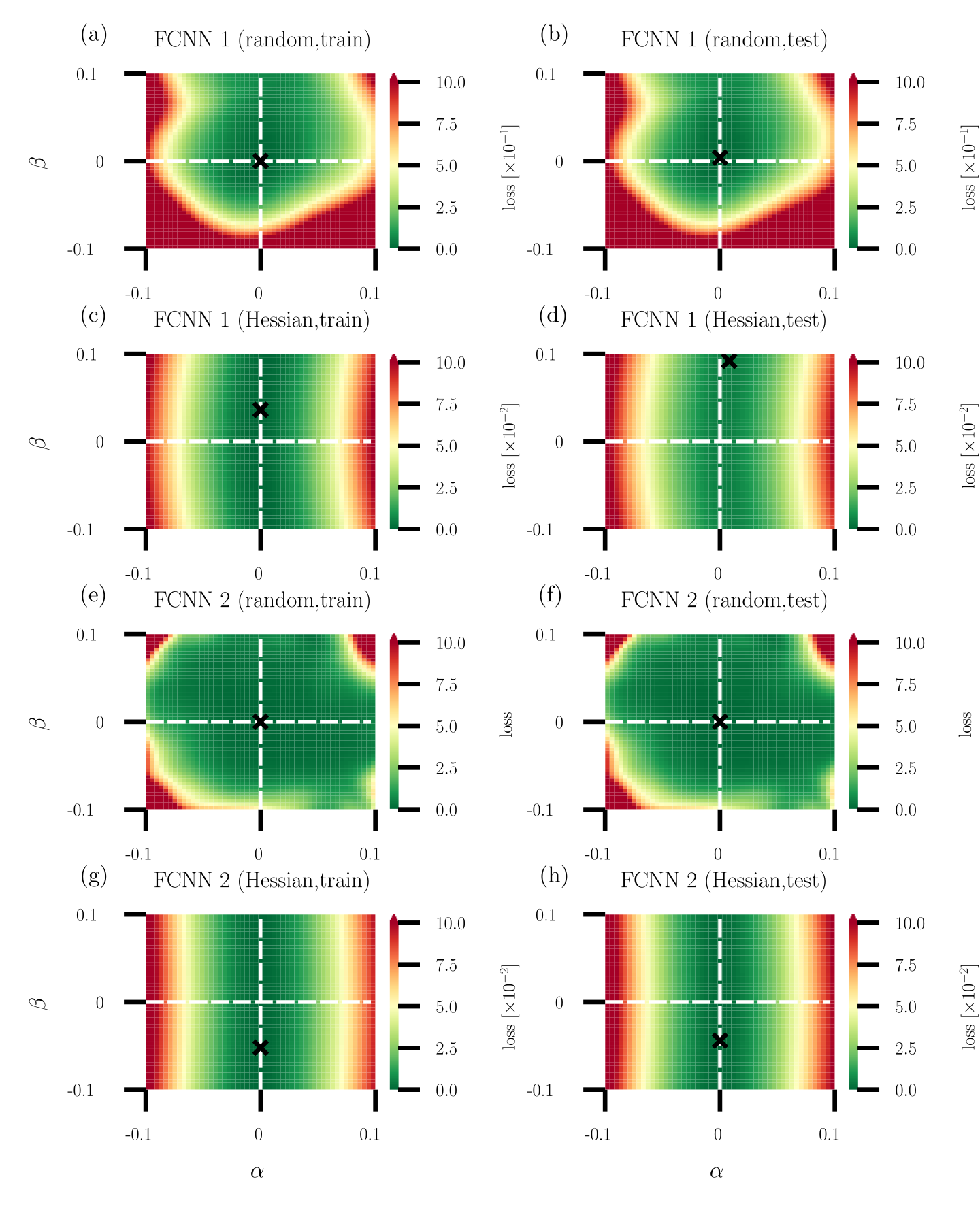
The image presents a series of heatmaps visualizing the loss landscapes of Fully Connected Neural Networks (FCNNs) under different training conditions and architectures. Each heatmap represents the loss value as a function of two parameters, alpha (α) and beta (β). The heatmaps are arranged in a 2x4 grid, varying by network architecture (FCNN 1 vs. FCNN 2), training method (random vs. Hessian), and dataset (train vs. test).
### Components/Axes
* **X-axis (Horizontal):** α (alpha), ranging from -0.1 to 0.1.
* **Y-axis (Vertical):** β (beta), ranging from -0.1 to 0.1.
* **Color Scale (Right):** Represents the loss value. The scale ranges from 0.0 to 10.0, with color transitions indicating different loss levels. Red indicates higher loss, and green indicates lower loss. The loss is scaled by 10^-1 for the top row and 10^-2 for the remaining rows.
* **Titles:** Each subplot has a title indicating the FCNN architecture (1 or 2), training method (random or Hessian), and dataset (train or test).
* (a) FCNN 1 (random, train)
* (b) FCNN 1 (random, test)
* (c) FCNN 1 (Hessian, train)
* (d) FCNN 1 (Hessian, test)
* (e) FCNN 2 (random, train)
* (f) FCNN 2 (random, test)
* (g) FCNN 2 (Hessian, train)
* (h) FCNN 2 (Hessian, test)
* **Axes Markers:** The axes are marked at -0.1, 0, and 0.1 for both α and β.
* **Crosshair:** Each plot contains a dashed white crosshair centered at (0,0). A black 'X' is located at the intersection of the crosshair.
### Detailed Analysis
**Subplot (a): FCNN 1 (random, train)**
* Trend: A green (low loss) region is centered around (0,0), surrounded by a red (high loss) region in the corners.
* Loss values: The minimum loss (green) is approximately 0 near the center. The maximum loss (red) reaches approximately 10 * 10^-1 = 1.0 in the corners.
**Subplot (b): FCNN 1 (random, test)**
* Trend: Similar to (a), a green (low loss) region is centered around (0,0), surrounded by a red (high loss) region in the corners.
* Loss values: The minimum loss (green) is approximately 0 near the center. The maximum loss (red) reaches approximately 10 * 10^-1 = 1.0 in the corners.
**Subplot (c): FCNN 1 (Hessian, train)**
* Trend: A horizontal green band (low loss) is centered around β = 0, with red regions (high loss) above and below.
* Loss values: The minimum loss (green) is approximately 0 along the horizontal band. The maximum loss (red) reaches approximately 10 * 10^-2 = 0.1 at the top and bottom edges.
**Subplot (d): FCNN 1 (Hessian, test)**
* Trend: Similar to (c), a horizontal green band (low loss) is centered around β = 0, with red regions (high loss) above and below.
* Loss values: The minimum loss (green) is approximately 0 along the horizontal band. The maximum loss (red) reaches approximately 10 * 10^-2 = 0.1 at the top and bottom edges.
**Subplot (e): FCNN 2 (random, train)**
* Trend: A green (low loss) region is centered around (0,0), with red regions (high loss) in the corners. The green region appears slightly more elongated vertically compared to FCNN 1.
* Loss values: The minimum loss (green) is approximately 0 near the center. The maximum loss (red) reaches approximately 10 * 10^-2 = 0.1 in the corners.
**Subplot (f): FCNN 2 (random, test)**
* Trend: Similar to (e), a green (low loss) region is centered around (0,0), with red regions (high loss) in the corners.
* Loss values: The minimum loss (green) is approximately 0 near the center. The maximum loss (red) reaches approximately 10 * 10^-2 = 0.1 in the corners.
**Subplot (g): FCNN 2 (Hessian, train)**
* Trend: A horizontal green band (low loss) is centered around β = 0, with red regions (high loss) above and below.
* Loss values: The minimum loss (green) is approximately 0 along the horizontal band. The maximum loss (red) reaches approximately 10 * 10^-2 = 0.1 at the top and bottom edges.
**Subplot (h): FCNN 2 (Hessian, test)**
* Trend: Similar to (g), a horizontal green band (low loss) is centered around β = 0, with red regions (high loss) above and below.
* Loss values: The minimum loss (green) is approximately 0 along the horizontal band. The maximum loss (red) reaches approximately 10 * 10^-2 = 0.1 at the top and bottom edges.
### Key Observations
* **Training Method Impact:** The Hessian training method results in a loss landscape with a clear horizontal band of low loss around β = 0 for both FCNN 1 and FCNN 2. The random training method results in a more localized low-loss region around (0,0).
* **Network Architecture Impact:** The loss landscapes for FCNN 1 and FCNN 2 are qualitatively similar for both random and Hessian training methods. However, the scale of the loss differs, with FCNN 1 (random) having a higher loss scale (10^-1) compared to the others (10^-2).
* **Train vs. Test:** The loss landscapes for train and test datasets are very similar for each combination of network architecture and training method, suggesting good generalization.
### Interpretation
The heatmaps visualize how the loss function changes as the parameters α and β are varied. The goal is to find the values of α and β that minimize the loss, represented by the green regions.
The Hessian training method appears to create a loss landscape where the loss is less sensitive to changes in α, as indicated by the horizontal bands of low loss. This might suggest that the Hessian method leads to a more robust solution with respect to variations in α.
The random training method, on the other hand, results in a more localized minimum around (0,0), suggesting that the solution is more sensitive to changes in both α and β.
The similarity between the train and test loss landscapes indicates that the models are generalizing well to unseen data. The difference in loss scale between FCNN 1 (random) and the other configurations suggests that FCNN 1 (random) might be less efficient or require further optimization.