## Heatmap Grid: Loss Landscapes for FCNN 1 and FCNN 2 under Different Training/Test Conditions
### Overview
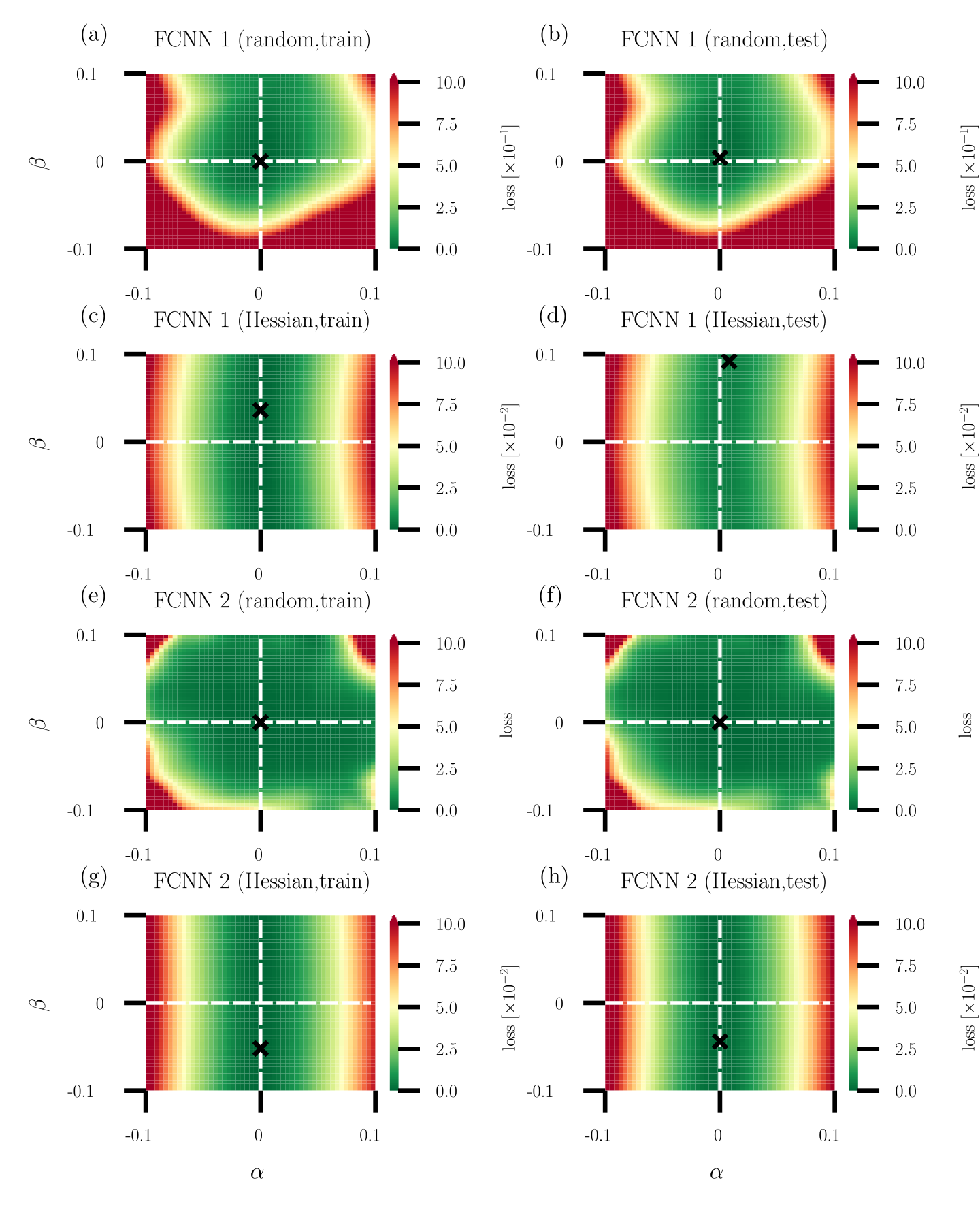
The image displays eight heatmaps arranged in a 4x2 grid, visualizing loss landscapes for two feedforward convolutional neural networks (FCNN 1 and FCNN 2) under varying training and testing conditions. Each heatmap uses a color gradient (green to red) to represent loss magnitude, with axes labeled α (horizontal) and β (vertical). A black "X" marks the optimal parameter combination (minimum loss) in each case.
---
### Components/Axes
1. **Axes**:
- **X-axis (α)**: Ranges from -0.1 to 0.1 in all heatmaps.
- **Y-axis (β)**: Ranges from -0.1 to 0.1 in all heatmaps.
- **Color Scale**: Loss values from 0.0 (green) to 10.0 (red), with intermediate steps at 2.5, 5.0, and 7.5.
2. **Labels**:
- **Top Row (a, b)**: FCNN 1 (random initialization).
- **Second Row (c, d)**: FCNN 1 (Hessian-based optimization).
- **Third Row (e, f)**: FCNN 2 (random initialization).
- **Bottom Row (g, h)**: FCNN 2 (Hessian-based optimization).
- **Sub-labels**:
- `(train)`: Training phase (left column: a, c, e, g).
- `(test)`: Testing phase (right column: b, d, f, h).
3. **Legend**:
- Color bar on the right of each heatmap maps loss values to colors (green = low loss, red = high loss).
---
### Detailed Analysis
#### FCNN 1 (Random Initialization)
- **(a) FCNN 1 (random, train)**:
- Loss landscape is smooth with a broad minimum centered near α=0, β=0.
- Loss values increase radially outward, peaking at ~10.0 in corners.
- **(b) FCNN 1 (random, test)**:
- Similar to (a) but with a slightly shifted minimum (α≈0.05, β≈-0.05).
- Loss values are marginally higher in the top-right quadrant.
#### FCNN 1 (Hessian Optimization)
- **(c) FCNN 1 (Hessian, train)**:
- Loss landscape is flatter with a concentrated minimum at α≈0.02, β≈-0.03.
- Loss values remain below 5.0 in most regions.
- **(d) FCNN 1 (Hessian, test)**:
- Minimum shifts to α≈0.03, β≈-0.02.
- Loss values are more uniform, with a sharp gradient near the optimal point.
#### FCNN 2 (Random Initialization)
- **(e) FCNN 2 (random, train)**:
- Loss landscape has a saddle-like structure with minima at α≈-0.05, β≈0.05 and α≈0.05, β≈-0.05.
- Loss values exceed 7.5 in the top-left and bottom-right quadrants.
- **(f) FCNN 2 (random, test)**:
- Minima shift to α≈-0.03, β≈0.03 and α≈0.03, β≈-0.03.
- Loss values are more concentrated but retain a bimodal distribution.
#### FCNN 2 (Hessian Optimization)
- **(g) FCNN 2 (Hessian, train)**:
- Loss landscape is nearly flat with a diffuse minimum at α≈0.01, β≈-0.01.
- Loss values remain below 3.0 across most regions.
- **(h) FCNN 2 (Hessian, test)**:
- Minimum sharpens to α≈0.02, β≈-0.02.
- Loss values show a clear gradient, with the lowest point at ~1.0.
---
### Key Observations
1. **Optimal Points (X)**:
- All heatmaps show the optimal parameter combination (X) near the center (α≈0, β≈0), but its exact position varies slightly between training and testing.
- Hessian-based methods (c, d, g, h) exhibit more precise minima compared to random initialization (a, b, e, f).
2. **Loss Distribution**:
- **Random Initialization**: Broader, more dispersed loss landscapes (e.g., a, e).
- **Hessian Optimization**: Sharper, more focused minima (e.g., c, g).
3. **Training vs. Testing**:
- Training heatmaps (a, c, e, g) generally show smoother gradients.
- Testing heatmaps (b, d, f, h) exhibit sharper transitions near the optimal point, suggesting overfitting in some cases (e.g., e vs. f).
---
### Interpretation
The data demonstrates that Hessian-based optimization methods produce more stable and concentrated loss landscapes compared to random initialization. This suggests:
- **Improved Generalization**: Hessian methods reduce parameter sensitivity, leading to more consistent performance during testing.
- **Training Efficiency**: The flatter landscapes in Hessian-trained models (c, g) may indicate faster convergence during training.
- **Overfitting Risk**: The sharper minima in testing heatmaps (d, h) could imply overfitting, though this is mitigated by the Hessian approach.
The consistent positioning of the optimal point near the center (α≈0, β≈0) across all heatmaps implies that the model's optimal parameters are inherently centered, but the optimization method critically influences the landscape's shape and stability.