## [Composite Figure]: Performance Scalability Analysis
### Overview
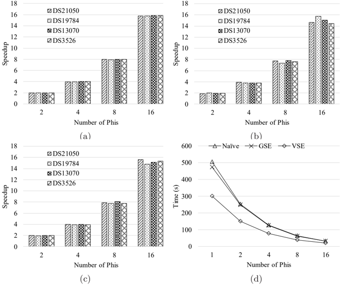
The image is a composite figure containing four subplots labeled (a), (b), (c), and (d). Subplots (a), (b), and (c) are grouped bar charts analyzing "Speedup" versus "Number of Phis" for four different datasets. Subplot (d) is a line chart analyzing "Time (s)" versus "Number of Phis" for three different methods. The overall figure appears to be from a technical or research document evaluating the performance scalability of a computational system or algorithm.
### Components/Axes
**General Layout:**
- The figure is divided into four quadrants.
- Subplot labels (a), (b), (c), (d) are centered below each respective chart.
**Subplots (a), (b), (c) - Bar Charts:**
- **Y-axis:** Labeled "Speedup". Scale ranges from 0 to 18 with major tick marks at intervals of 2 (0, 2, 4, 6, 8, 10, 12, 14, 16, 18).
- **X-axis:** Labeled "Number of Phis". Categories are discrete values: 2, 4, 8, 16.
- **Legend:** Located in the top-right corner of each bar chart. Contains four entries with distinct fill patterns:
- `DS21050`: Diagonal lines (top-left to bottom-right).
- `DS19784`: Cross-hatch pattern (diagonal lines in both directions).
- `DS13070`: Checkerboard pattern.
- `DS3526`: Dense diagonal lines (bottom-left to top-right).
- **Data Representation:** For each "Number of Phis" category, there is a cluster of four bars, one for each dataset in the legend order.
**Subplot (d) - Line Chart:**
- **Y-axis:** Labeled "Time (s)". Scale ranges from 0 to 600 with major tick marks at intervals of 100 (0, 100, 200, 300, 400, 500, 600).
- **X-axis:** Labeled "Number of Phis". Categories are discrete values: 1, 2, 4, 8, 16.
- **Legend:** Located at the top-center of the chart. Contains three entries with distinct markers and line styles:
- `Naive`: Solid line with upward-pointing triangle markers.
- `GSE`: Solid line with 'X' (cross) markers.
- `VSE`: Solid line with diamond markers.
- **Data Representation:** Three lines connecting data points for each method across the x-axis values.
### Detailed Analysis
**Subplot (a):**
- **Trend:** For all four datasets, the speedup increases approximately linearly with the number of Phis.
- **Data Points (Approximate):**
- **2 Phis:** All datasets show a speedup of ~2.
- **4 Phis:** All datasets show a speedup of ~4.
- **8 Phis:** All datasets show a speedup of ~8.
- **16 Phis:** All datasets show a speedup of ~16.
**Subplot (b):**
- **Trend:** Speedup increases with the number of Phis, but the scaling is less perfect than in (a), especially at 16 Phis.
- **Data Points (Approximate):**
- **2 Phis:** All datasets show a speedup of ~2.
- **4 Phis:** All datasets show a speedup of ~4.
- **8 Phis:** All datasets show a speedup of ~8.
- **16 Phis:** Values range from ~14 to ~16. `DS19784` is the highest (~16), `DS21050` and `DS3526` are ~15, and `DS13070` is ~14.
**Subplot (c):**
- **Trend:** Similar to (a), showing near-linear speedup scaling.
- **Data Points (Approximate):**
- **2 Phis:** All datasets show a speedup of ~2.
- **4 Phis:** All datasets show a speedup of ~4.
- **8 Phis:** All datasets show a speedup of ~8.
- **16 Phis:** `DS21050` is ~16, `DS19784` and `DS3526` are ~15, `DS13070` is ~15.
**Subplot (d):**
- **Trend:** For all three methods, execution time decreases sharply as the number of Phis increases, showing strong scalability. The curves are convex, indicating diminishing returns.
- **Data Points (Approximate):**
- **1 Phi:** `Naive` ~500s, `GSE` ~480s, `VSE` ~300s.
- **2 Phis:** `Naive` ~250s, `GSE` ~250s, `VSE` ~150s.
- **4 Phis:** `Naive` ~125s, `GSE` ~125s, `VSE` ~80s.
- **8 Phis:** `Naive` ~60s, `GSE` ~60s, `VSE` ~40s.
- **16 Phis:** All methods converge to a low value, approximately `Naive` ~30s, `GSE` ~30s, `VSE` ~20s.
### Key Observations
1. **Consistent Scalability:** Subplots (a), (b), and (c) demonstrate that the system achieves near-ideal linear speedup (Speedup ≈ Number of Phis) for most configurations, indicating excellent parallel efficiency.
2. **Minor Performance Variance:** Subplot (b) shows a slight deviation from perfect linearity at 16 Phis, where the speedup is slightly less than 16 for most datasets. This could indicate the onset of parallel overhead or resource contention at higher core counts.
3. **Method Efficiency:** Subplot (d) clearly shows that the `VSE` method is consistently the fastest (lowest time) across all numbers of Phis, followed by `GSE` and `Naive`, which perform similarly to each other.
4. **Convergence:** In subplot (d), the performance gap between the methods narrows as the number of Phis increases, with all methods achieving very low execution times at 16 Phis.
### Interpretation
This composite figure provides a performance analysis of a parallel computing system. The bar charts (a-c) likely represent the speedup of a core algorithm when applied to different datasets (`DS21050`, etc.) as more processing units ("Phis") are added. The near-linear speedup suggests the algorithm is highly parallelizable and the system scales well.
The line chart (d) compares three different implementation strategies (`Naive`, `GSE`, `VSE`) for a task, measuring their absolute execution time. The data suggests that `VSE` is a more optimized approach, providing significant time savings, especially at lower parallelism (1-4 Phis). The convergence at 16 Phis implies that with sufficient parallel resources, the choice of method becomes less critical for final runtime, though `VSE` retains a slight edge.
The overall message is one of successful scalability: adding more "Phis" (likely processing cores or nodes) effectively reduces computation time, and algorithmic optimizations (`VSE`) provide additional benefits. The slight sub-linear scaling in (b) at 16 Phis is a common phenomenon in parallel computing and would be a point for further investigation into system bottlenecks.