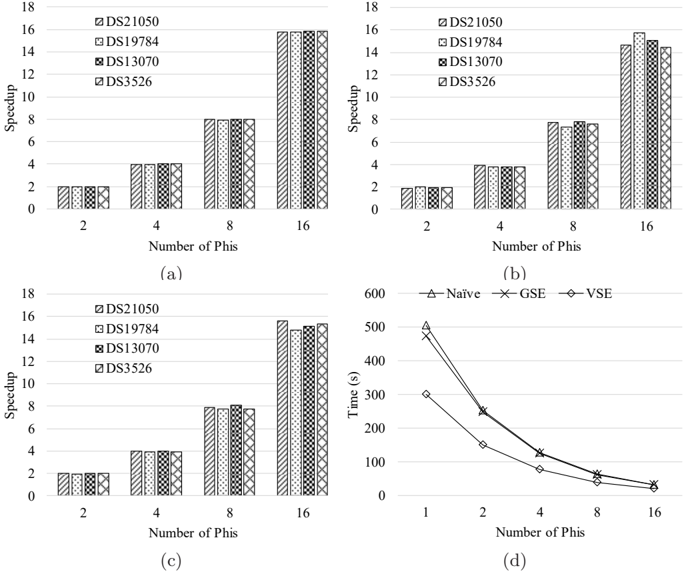
## Bar Charts and Line Graphs: Speedup and Time Analysis Across Datasets and Methods ### Overview The image contains four subplots analyzing computational performance metrics. Subplots (a), (b), and (c) are bar charts comparing speedup and time across datasets (DS21050, DS19784, DS13070, DS3526) at varying numbers of PHIs (2, 4, 8, 16). Subplot (d) is a line graph comparing time efficiency of three methods (Naïve, GSE, VSE) across PHI counts. All values are approximate with visual uncertainty. --- ### Components/Axes #### Subplot (a) - **X-axis**: Number of PHIs (2, 4, 8, 16) - **Y-axis**: Speedup (0–18) - **Legend**: - DS21050 (solid black) - DS19784 (dotted black) - DS13070 (crosshatch black) - DS3526 (diagonal stripes black) - **Legend Position**: Top-right #### Subplot (b) - **X-axis**: Number of PHIs (2, 4, 8, 16) - **Y-axis**: Speedup (0–18) - **Legend**: Same as (a) - **Legend Position**: Top-right #### Subplot (c) - **X-axis**: Number of PHIs (2, 4, 8, 16) - **Y-axis**: Time (s) (0–600) - **Legend**: Same as (a) - **Legend Position**: Top-right #### Subplot (d) - **X-axis**: Number of PHIs (1, 2, 4, 8, 16) - **Y-axis**: Time (s) (0–600) - **Legend**: - Naïve (triangle) - GSE (cross) - VSE (diamond) - **Legend Position**: Top-right --- ### Detailed Analysis #### Subplot (a) - **DS21050**: Speedup increases from ~2 (2 PHIs) to ~16 (16 PHIs). - **DS19784**: Speedup peaks at ~14 (16 PHIs), with ~4 at 4 PHIs. - **DS13070**: Speedup rises to ~12 (16 PHIs), ~3 at 4 PHIs. - **DS3526**: Speedup plateaus at ~2 across all PHI counts. #### Subplot (b) - **DS21050**: Speedup reaches ~14 (16 PHIs), ~2 at 2 PHIs. - **DS19784**: Speedup peaks at ~16 (16 PHIs), ~3 at 4 PHIs. - **DS13070**: Speedup ~12 (16 PHIs), ~4 at 8 PHIs. - **DS3526**: Speedup ~8 (16 PHIs), ~2 at 2 PHIs. #### Subplot (c) - **DS21050**: Time ~200s (2 PHIs) to ~140s (16 PHIs). - **DS19784**: Time ~400s (2 PHIs) to ~120s (16 PHIs). - **DS13070**: Time ~300s (2 PHIs) to ~100s (16 PHIs). - **DS3526**: Time ~500s (2 PHIs) to ~80s (16 PHIs). #### Subplot (d) - **Naïve**: Time decreases from ~500s (1 PHI) to ~50s (16 PHIs). - **GSE**: Time drops from ~450s (1 PHI) to ~40s (16 PHIs). - **VSE**: Time reduces from ~400s (1 PHI) to ~30s (16 PHIs). --- ### Key Observations 1. **Speedup Trends**: - DS21050 and DS19784 show the highest speedup gains with increasing PHIs. - DS3526 exhibits minimal speedup improvement, suggesting inefficiency or saturation. 2. **Time Efficiency**: - All methods improve time efficiency with more PHIs, but VSE outperforms others consistently. - Naïve method has the highest time overhead, especially at low PHI counts. 3. **Dataset Variability**: - DS3526 underperforms in speedup but achieves the lowest time in (c), indicating potential trade-offs. --- ### Interpretation - **Speedup vs. Time Trade-off**: Higher PHI counts generally improve speedup but reduce time, except for DS3526, which shows inconsistent behavior. - **Method Efficiency**: VSE is the most efficient method, reducing time by ~90% compared to Naïve at 16 PHIs. - **Dataset-Specific Behavior**: DS21050 and DS19784 benefit most from PHI scaling, while DS3526 may have architectural or algorithmic limitations. - **Anomalies**: DS3526’s low speedup in (a) contrasts with its low time in (c), suggesting it may prioritize throughput over latency or vice versa. This analysis highlights the importance of method selection (VSE) and dataset characteristics in optimizing computational performance.