\n
## Box Plot: NSGA-II with N=n+1 on OneMinMax
### Overview
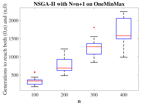
The image displays a box plot chart titled "NSGA-II with N=n+1 on OneMinMax". It visualizes the distribution of the number of generations required for an algorithm (NSGA-II with population size N=n+1) to solve the "OneMinMax" problem for different problem sizes (n). The chart shows a clear positive correlation between the problem size `n` and the computational effort (generations) required.
### Components/Axes
* **Chart Title:** "NSGA-II with N=n+1 on OneMinMax" (Top Center).
* **Y-Axis Label:** "Generations to reach both (0,n) and (n,0)" (Left side, vertical text). This indicates the metric is the number of generations needed to find both optimal solutions for the bi-objective problem.
* **X-Axis Label:** "n" (Bottom Center). Represents the problem size parameter.
* **X-Axis Categories/Ticks:** Four discrete values: `100`, `200`, `300`, `400`.
* **Plot Elements:** For each `n`, a standard box-and-whisker plot is shown.
* **Blue Box:** Represents the interquartile range (IQR), from the 25th percentile (Q1) to the 75th percentile (Q3).
* **Red Line:** Inside each box marks the median (50th percentile).
* **Black Dashed Whiskers:** Extend from the box to the minimum and maximum data points within 1.5 * IQR.
* **Red Plus Signs (+):** Indicate individual outlier data points beyond the whiskers.
### Detailed Analysis
The following table summarizes the approximate key values extracted from each box plot. Values are estimated from the visual chart and carry inherent uncertainty.
| n | Median (Red Line) | IQR (Blue Box) Range (Approx.) | Full Range (Whiskers, Approx.) | Outlier(s) (Red +) |
| :-- | :---------------- | :----------------------------- | :----------------------------- | :----------------- |
| 100 | ~300 | 250 to 350 | 200 to 400 | ~600 |
| 200 | ~700 | 600 to 900 | 500 to 1200 | None visible |
| 300 | ~1200 | 1000 to 1400 | 800 to 1600 | ~1800 |
| 400 | ~1600 | 1500 to 2000 | 1000 to 2200 | None visible |
**Trend Verification:**
* **Visual Trend:** For each successive data series (from n=100 to n=400), the entire box plot (median, IQR, and whiskers) shifts upward on the y-axis. This confirms a strong, positive, monotonic trend: as `n` increases, the number of generations required increases significantly.
* **Spread Trend:** The vertical size of the blue boxes (IQR) and the length of the whiskers generally increase with `n`, indicating greater variability in the algorithm's performance for larger problem sizes.
### Key Observations
1. **Clear Scaling Relationship:** The median generations required scales approximately linearly with `n`. The median roughly doubles when `n` doubles from 100 to 200 (~300 to ~700), and again from 200 to 400 (~700 to ~1600).
2. **Increasing Variability:** The interquartile range (IQR) widens as `n` increases. For n=100, the IQR spans ~100 generations. For n=400, it spans ~500 generations. This suggests the algorithm's runtime becomes less predictable for larger problems.
3. **Presence of Outliers:** High-value outliers are present for n=100 (~600) and n=300 (~1800). These represent specific runs where the algorithm took significantly longer than typical. No outliers are visible for n=200 or n=400 within the plotted range.
4. **Minimum Performance Floor:** Even the fastest runs (bottom whisker) require more generations as `n` grows. The minimum observed generations for n=400 (~1000) is higher than the *median* for n=200 (~700).
### Interpretation
This chart demonstrates the **computational complexity** of the NSGA-II algorithm when applied to the OneMinMax problem with a population size scaled as N=n+1. The data suggests:
* **Problem Difficulty Scales with `n`:** The OneMinMax problem becomes harder for NSGA-II to solve as the problem dimension `n` increases, requiring more generations on average. The near-linear scaling of the median is a key performance characteristic.
* **Algorithmic Stability Decreases:** The increasing spread (IQR) indicates that for larger `n`, the algorithm's performance is more sensitive to initial conditions or stochastic elements, leading to a wider range of possible runtimes.
* **Practical Implication:** For a practitioner, this means that solving larger instances of this problem (e.g., n=400) will not only take longer on average but will also have a less predictable completion time. Planning for resources would require considering the upper quartile or whisker values, not just the median.
* **Underlying Pattern:** The relationship visualized here is a direct empirical measurement of the algorithm's time complexity for this specific problem configuration. It provides concrete data to compare against theoretical models or other algorithms.