## Chart/Diagram Type: Four Scatter Plots
### Overview
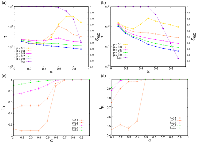
The image contains four scatter plots, arranged in a 2x2 grid. Each plot displays the relationship between two variables, with different line colors representing different parameter values. The plots explore how these relationships change under varying conditions.
### Components/Axes
**General Components:**
* Each plot has an x-axis labeled "α" ranging from 0 to 1, with tick marks at intervals of 0.2.
* Each plot has a legend indicating the parameter "p" with values 0.1, 0.3, 0.5, 0.7, and 0.9. The legend also includes a data series labeled "SGC".
* The plots are labeled (a), (b), (c), and (d) in the top-left corner of each plot.
**Plot (a):**
* Y-axis (left): "τ" (tau), with a logarithmic scale ranging from 10^1 to 10^3.
* Y-axis (right): "SGC", with a linear scale ranging from 0.9 to 1.
* Data series:
* p = 0.1 (yellow): Approximately constant at τ ≈ 20.
* p = 0.3 (orange): Approximately constant at τ ≈ 15.
* p = 0.5 (pink): Approximately constant at τ ≈ 13.
* p = 0.7 (green): Approximately constant at τ ≈ 12.
* p = 0.9 (blue): Decreases slightly from τ ≈ 11 to τ ≈ 10.
* SGC (purple, dashed): Decreases from SGC ≈ 1 to SGC ≈ 0.97.
**Plot (b):**
* Y-axis (left): "τ" (tau), with a logarithmic scale ranging from 10^0 to 10^3.
* Y-axis (right): "SGC", with a linear scale ranging from 0.1 to 1.
* Data series:
* p = 0.1 (yellow): Decreases from τ ≈ 150 to τ ≈ 20.
* p = 0.3 (orange): Decreases from τ ≈ 100 to τ ≈ 15.
* p = 0.5 (pink): Decreases from τ ≈ 60 to τ ≈ 12.
* p = 0.7 (green): Decreases from τ ≈ 40 to τ ≈ 10.
* p = 0.9 (blue): Decreases from τ ≈ 25 to τ ≈ 8.
* SGC (purple, dashed): Decreases from SGC ≈ 1 to SGC ≈ 0.1.
**Plot (c):**
* Y-axis: "fR", with a linear scale ranging from 0 to 1.
* Data series:
* p = 0.1 (yellow): Increases from fR ≈ 0.1 to fR ≈ 1 around α = 0.6.
* p = 0.3 (orange): Increases from fR ≈ 0.1 to fR ≈ 1 around α = 0.5.
* p = 0.5 (pink): Increases from fR ≈ 0.7 to fR ≈ 1 around α = 0.6.
* p = 0.7 (green): Constant at fR ≈ 1.
* p = 0.9 (blue): Constant at fR ≈ 1.
**Plot (d):**
* Y-axis: "fR", with a linear scale ranging from 0.4 to 1.
* Data series:
* p = 0.1 (yellow): Increases from fR ≈ 0.45 to fR ≈ 1 around α = 0.5.
* p = 0.3 (orange): Increases from fR ≈ 0.45 to fR ≈ 1 around α = 0.4.
* p = 0.5 (pink): Constant at fR ≈ 1.
* p = 0.7 (green): Constant at fR ≈ 1.
* p = 0.9 (blue): Constant at fR ≈ 1.
### Detailed Analysis or ### Content Details
**Plot (a):**
* The lines for p = 0.1, 0.3, 0.5, and 0.7 are relatively flat, indicating that τ is nearly constant with respect to α for these values of p.
* The line for p = 0.9 shows a slight decrease in τ as α increases.
* The SGC line decreases as α increases.
**Plot (b):**
* All lines for p = 0.1, 0.3, 0.5, 0.7, and 0.9 show a decrease in τ as α increases.
* The SGC line decreases as α increases.
**Plot (c):**
* The lines for p = 0.1 and 0.3 show a sharp increase in fR as α increases.
* The lines for p = 0.5, 0.7, and 0.9 are relatively constant at fR ≈ 1.
**Plot (d):**
* The lines for p = 0.1 and 0.3 show a sharp increase in fR as α increases.
* The lines for p = 0.5, 0.7, and 0.9 are relatively constant at fR ≈ 1.
### Key Observations
* Plots (a) and (b) show the relationship between τ and α, while plots (c) and (d) show the relationship between fR and α.
* The parameter p affects the behavior of τ and fR as α changes.
* The SGC value decreases as α increases in plots (a) and (b).
* In plots (c) and (d), fR tends to increase as α increases, especially for lower values of p.
### Interpretation
The plots illustrate how different parameters (p and α) influence the variables τ, fR, and SGC. The data suggests that:
* **τ (tau)**: In plot (a), τ remains relatively constant with respect to α for higher values of p (0.1 to 0.7), while it decreases slightly for p = 0.9. In plot (b), τ decreases as α increases for all values of p. This suggests that the relationship between τ and α is dependent on the specific conditions being modeled.
* **fR**: In plots (c) and (d), fR generally increases as α increases, particularly for lower values of p (0.1 and 0.3). This indicates a threshold effect, where fR rapidly increases once α reaches a certain value.
* **SGC**: In plots (a) and (b), SGC decreases as α increases. This suggests an inverse relationship between SGC and α.
The differences between plots (a)/(b) and (c)/(d) likely represent different aspects or regimes of the system being studied. The parameter 'p' seems to control the sensitivity of the system to changes in 'α', with lower 'p' values leading to more pronounced transitions in 'fR' as 'α' increases. The logarithmic scale on the y-axis of plots (a) and (b) indicates that 'τ' can vary over several orders of magnitude, highlighting its sensitivity to the parameters.