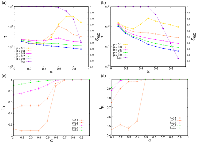
\n ## Charts: Parameter Variation Analysis ### Overview The image contains four separate charts (labeled a, b, c, and d) displaying the relationship between a parameter α (ranging from 0 to 1) and various metrics: τ, SGC, rR, and fR. Each chart also shows the impact of varying a parameter 'p' (with values 0.1, 0.3, 0.5, 0.7, and 0.9) on these metrics. Charts (a) and (b) have a dual y-axis, one linear and one logarithmic. Charts (b) and (d) also include a secondary y-axis representing SGC. ### Components/Axes * **X-axis (all charts):** α (Alpha), ranging from 0 to 1. * **Y-axis (a):** τ (Tau), logarithmic scale from 10^0 to 10^3. * **Y-axis (b):** SGC (left axis), logarithmic scale from 10^0 to 10^3; α (right axis), linear scale from 0.9 to 1. * **Y-axis (c):** rR (R squared), linear scale from 0 to 1. * **Y-axis (d):** fR (F measure), linear scale from 0.4 to 1. * **Legend (all charts):** p = 0.1 (blue), p = 0.3 (green), p = 0.5 (red), p = 0.7 (orange), p = 0.9 (purple), SGC (dashed black). ### Detailed Analysis or Content Details **Chart (a): τ vs. α** * **p = 0.1 (blue):** Line is relatively flat, starting at approximately τ = 20 and ending at approximately τ = 25. * **p = 0.3 (green):** Line starts at approximately τ = 20, dips to approximately τ = 15 at α = 0.2, then rises to approximately τ = 25 at α = 1. * **p = 0.5 (red):** Line starts at approximately τ = 20, rises to approximately τ = 40 at α = 0.4, then decreases to approximately τ = 25 at α = 1. * **p = 0.7 (orange):** Line starts at approximately τ = 20, rises to approximately τ = 100 at α = 0.8, then drops to approximately τ = 25 at α = 1. * **p = 0.9 (purple):** Line is relatively flat, starting at approximately τ = 20 and ending at approximately τ = 20. * **SGC (dashed black):** Line is relatively flat, starting at approximately SGC = 0.99 and ending at approximately SGC = 0.99. **Chart (b): SGC vs. α** * **p = 0.1 (blue):** Line slopes downward, starting at approximately SGC = 0.98 and ending at approximately SGC = 0.92. * **p = 0.3 (green):** Line slopes downward, starting at approximately SGC = 0.98 and ending at approximately SGC = 0.93. * **p = 0.5 (red):** Line slopes downward, starting at approximately SGC = 0.98 and ending at approximately SGC = 0.92. * **p = 0.7 (orange):** Line slopes downward, starting at approximately SGC = 0.98 and ending at approximately SGC = 0.91. * **p = 0.9 (purple):** Line slopes downward, starting at approximately SGC = 0.98 and ending at approximately SGC = 0.91. * **SGC (dashed black):** Line is relatively flat, starting at approximately SGC = 100 and ending at approximately SGC = 100. **Chart (c): rR vs. α** * **p = 0.1 (blue):** Line is relatively flat, starting at approximately rR = 0.2 and ending at approximately rR = 0.2. * **p = 0.3 (green):** Line increases steadily, starting at approximately rR = 0.2 and ending at approximately rR = 0.8. * **p = 0.5 (red):** Line increases steadily, starting at approximately rR = 0.2 and ending at approximately rR = 0.9. * **p = 0.7 (orange):** Line increases rapidly, starting at approximately rR = 0.2 and ending at approximately rR = 0.8. * **p = 0.9 (purple):** Line increases rapidly, starting at approximately rR = 0.2 and ending at approximately rR = 0.9. **Chart (d): fR vs. α** * **p = 0.1 (blue):** Line is relatively flat, starting at approximately fR = 0.5 and ending at approximately fR = 0.5. * **p = 0.3 (green):** Line increases rapidly, starting at approximately fR = 0.4 and ending at approximately fR = 0.9. * **p = 0.5 (red):** Line increases rapidly, starting at approximately fR = 0.4 and ending at approximately fR = 0.9. * **p = 0.7 (orange):** Line increases slowly, starting at approximately fR = 0.4 and ending at approximately fR = 0.6. * **p = 0.9 (purple):** Line increases rapidly, starting at approximately fR = 0.4 and ending at approximately fR = 0.9. ### Key Observations * In charts (a) and (b), the SGC remains relatively constant, while τ decreases with increasing α for p > 0.1. * Charts (c) and (d) show a clear trend of increasing rR and fR with increasing α, particularly for higher values of p (0.5, 0.7, and 0.9). * The parameter 'p' significantly influences the behavior of τ, SGC, rR, and fR. * The behavior of τ is most sensitive to changes in α when p is 0.5 and 0.7. ### Interpretation These charts likely represent the performance of a model or algorithm as its parameters (α and p) are varied. α could represent a regularization parameter, while p might control some aspect of the data or model complexity. * **Charts (a) and (b):** The relatively constant SGC suggests that the model's overall structure or stability is maintained across different values of α. The decrease in τ with increasing α (for p > 0.1) could indicate a reduction in model complexity or overfitting. * **Charts (c) and (d):** The increasing rR and fR with increasing α suggest that the model's predictive power and accuracy improve as α increases, especially for higher values of p. This could be because higher α values allow the model to better capture the underlying patterns in the data. * The different behaviors observed for different values of p suggest that the optimal value of α depends on the specific context or data being used. The combination of these observations suggests that there is a trade-off between model complexity and performance. Increasing α can improve predictive power, but it may also lead to overfitting if p is too low. The optimal value of α depends on the specific characteristics of the data and the desired level of model complexity. The SGC metric appears to be a measure of model stability, and its relatively constant value suggests that the model is robust to changes in α.