## Line Graphs: Relationships Between Parameters Across Four Subplots
### Overview
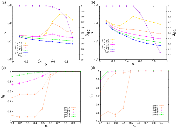
The image contains four line graphs (a-d) arranged in a 2x2 grid, analyzing relationships between parameters α (x-axis) and τ/f_R (y-axes) under varying probabilities (p). All graphs use logarithmic scales for τ in (a) and (b), while (c) and (d) use linear scales. Key elements include legends, reference lines (S_GC), and error bars in (c) and (d).
---
### Components/Axes
#### Subplot (a): τ vs α
- **X-axis**: α (0 to 1, linear scale)
- **Y-axis**: τ (10⁰ to 10³, log scale)
- **Legend**: p = 0.1 (orange), 0.3 (red), 0.5 (pink), 0.7 (green), 0.9 (blue), S_GC (purple dotted line)
- **Spatial Grounding**: Legend on right; S_GC line spans entire α range.
#### Subplot (b): S_GC vs τ
- **X-axis**: τ (10⁰ to 10³, log scale)
- **Y-axis**: S_GC (0.1 to 1, linear scale)
- **Legend**: Same p values as (a), with S_GC (purple dotted line)
- **Spatial Grounding**: Legend on right; S_GC line slopes downward.
#### Subplot (c): f_R vs α
- **X-axis**: α (0.1 to 1, linear scale)
- **Y-axis**: f_R (0 to 1, linear scale)
- **Legend**: p = 0.1 (orange), 0.3 (red), 0.5 (pink), 0.7 (green), 0.9 (blue)
- **Spatial Grounding**: Legend on right; error bars visible for p=0.1 and 0.3.
#### Subplot (d): f_R vs α (Zoomed View)
- **X-axis**: α (0.1 to 1, linear scale)
- **Y-axis**: f_R (0.4 to 1, linear scale)
- **Legend**: Same p values as (c)
- **Spatial Grounding**: Legend on right; error bars only for p=0.1.
---
### Detailed Analysis
#### Subplot (a): τ vs α
- **Trends**:
- τ peaks at α ≈ 0.5 for p=0.1 (≈100) and p=0.3 (≈150), then declines.
- p=0.9 (blue) shows minimal τ (~10) across all α.
- S_GC (purple) remains constant at ~1000.
- **Data Points**:
- p=0.1: τ ≈ 100 at α=0.5; ~10 at α=1.
- p=0.9: τ ≈ 10 at α=0.1; ~5 at α=1.
#### Subplot (b): S_GC vs τ
- **Trends**:
- S_GC decreases with τ for all p values.
- p=0.1 (orange) starts at ~0.98 (τ=10) and drops to ~0.7 (τ=1000).
- p=0.9 (blue) declines from ~0.95 to ~0.3.
- S_GC (purple) remains flat at ~0.9.
#### Subplot (c): f_R vs α
- **Trends**:
- f_R increases sharply with α for lower p values.
- p=0.1 (orange) rises from ~0.1 (α=0.1) to ~0.8 (α=1).
- p=0.9 (green) stays near 0.9 across all α.
- **Data Points**:
- p=0.1: f_R ≈ 0.2 at α=0.3; ~0.8 at α=1.
- p=0.7: f_R ≈ 0.7 at α=0.5; ~0.9 at α=1.
#### Subplot (d): f_R vs α (Zoomed View)
- **Trends**:
- Similar to (c), but focuses on α=0.1–0.5.
- p=0.1 (orange) jumps from ~0.5 (α=0.4) to ~0.8 (α=0.5).
- p=0.3 (red) shows smaller increments (~0.5 to ~0.6).
---
### Key Observations
1. **τ and p**: Higher p values correlate with lower τ (e.g., p=0.9 has τ ~10 vs. p=0.1’s ~100 at α=0.5).
2. **S_GC**: Inversely related to τ; higher τ reduces S_GC (e.g., p=0.1’s S_GC drops from 0.98 to 0.7 as τ increases).
3. **f_R**: Increases with α, especially for lower p. p=0.1 shows the steepest rise (~0.1 to 0.8), while p=0.9 remains stable (~0.9).
4. **Error Bars**: Larger uncertainties in f_R for p=0.1 and 0.3 in (c) and (d).
---
### Interpretation
- **Parameter Interactions**: τ and S_GC are inversely related, suggesting a trade-off between these metrics. Higher p values reduce τ but also lower S_GC, indicating diminishing returns.
- **f_R Dynamics**: f_R’s sensitivity to α is p-dependent. Lower p values (e.g., 0.1) exhibit nonlinear growth, while higher p values (e.g., 0.9) plateau, implying system stability at high probabilities.
- **S_GC as Threshold**: The constant S_GC line (~0.9) may represent a critical system boundary, with deviations indicating performance thresholds.
- **Anomalies**: The sharp rise in f_R for p=0.1 at α=0.5 (subplot d) suggests a phase transition or critical point in the system’s behavior.
This analysis highlights how α and p jointly influence system performance, with implications for optimizing parameters in probabilistic models.