## Density Plot: Cosine Similarity Distribution
### Overview
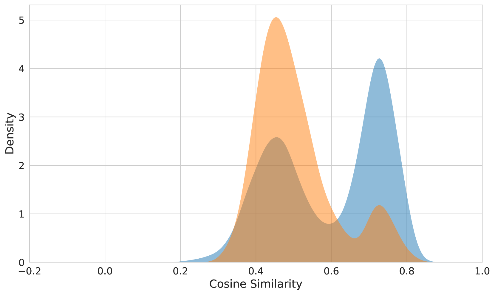
The image is a density plot showing the distribution of cosine similarity scores. Two overlapping distributions are displayed, one in light blue and the other in light orange. The x-axis represents cosine similarity, ranging from -0.2 to 1.0, and the y-axis represents density, ranging from 0 to 5.
### Components/Axes
* **X-axis:** Cosine Similarity, ranging from -0.2 to 1.0 with increments of 0.2.
* **Y-axis:** Density, ranging from 0 to 5 with increments of 1.
* **Distributions:** Two distributions are plotted:
* Light Blue Distribution: Peaks around a cosine similarity of approximately 0.75.
* Light Orange Distribution: Peaks around a cosine similarity of approximately 0.45.
### Detailed Analysis
* **Light Blue Distribution:**
* Starts around a cosine similarity of 0.2.
* Rises to a peak density of approximately 4.2 at a cosine similarity of 0.75.
* Decreases back to near 0 density by a cosine similarity of 0.9.
* **Light Orange Distribution:**
* Starts around a cosine similarity of 0.2.
* Rises to a peak density of approximately 5.1 at a cosine similarity of 0.45.
* Decreases to a density of approximately 1 at a cosine similarity of 0.7.
### Key Observations
* The light orange distribution has a higher peak density (approximately 5.1) compared to the light blue distribution (approximately 4.2).
* The light orange distribution is centered around a lower cosine similarity value (approximately 0.45) compared to the light blue distribution (approximately 0.75).
* There is an overlap between the two distributions in the cosine similarity range of approximately 0.3 to 0.7.
### Interpretation
The density plot visualizes the distribution of cosine similarity scores for two different datasets or categories. The light orange distribution indicates a higher concentration of data points with lower cosine similarity values, while the light blue distribution indicates a higher concentration of data points with higher cosine similarity values. The overlap suggests that there are some data points that share similar cosine similarity values between the two distributions. This could indicate a degree of similarity or overlap between the two categories being compared. The difference in peak densities and locations suggests that the two categories have distinct characteristics in terms of cosine similarity.