## Density Plots: Sum of Existence Weights
### Overview
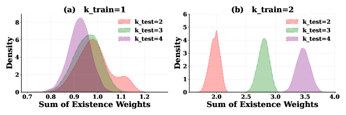
The image contains two density plots, labeled (a) and (b), showing the distribution of "Sum of Existence Weights" for different values of `k_test` (2, 3, and 4) when `k_train` is set to 1 (plot a) and 2 (plot b). The x-axis represents the "Sum of Existence Weights," and the y-axis represents the "Density."
### Components/Axes
* **Plot (a) Title:** (a) k\_train=1
* **Plot (b) Title:** (b) k\_train=2
* **X-axis Title (both plots):** Sum of Existence Weights
* **Y-axis Title (both plots):** Density
* **Y-axis Scale (Plot a):** 0 to 8, with ticks at 0, 2, 4, 6, and 8.
* **Y-axis Scale (Plot b):** 0 to 6, with ticks at 0, 1, 2, 3, 4, 5, and 6.
* **X-axis Scale (Plot a):** 0.7 to 1.2, with ticks at 0.7, 0.8, 0.9, 1.0, 1.1, and 1.2.
* **X-axis Scale (Plot b):** 2.0 to 4.0, with ticks at 2.0, 2.5, 3.0, 3.5, and 4.0.
* **Legend (both plots, located in the top-right):**
* k\_test=2 (light red)
* k\_test=3 (light green)
* k\_test=4 (light purple)
### Detailed Analysis
**Plot (a): k\_train=1**
* **k\_test=2 (light red):** The distribution is unimodal, with a peak around 1.0. It extends from approximately 0.8 to 1.2.
* **k\_test=3 (light green):** The distribution is unimodal, with a peak around 0.95. It extends from approximately 0.8 to 1.1.
* **k\_test=4 (light purple):** The distribution is unimodal, with a peak around 0.9. It extends from approximately 0.75 to 1.05.
**Plot (b): k\_train=2**
* **k\_test=2 (light red):** The distribution is unimodal, with a peak around 2.0. It extends from approximately 1.75 to 2.25.
* **k\_test=3 (light green):** The distribution is unimodal, with a peak around 2.8. It extends from approximately 2.5 to 3.0.
* **k\_test=4 (light purple):** The distribution is unimodal, with a peak around 3.5. It extends from approximately 3.25 to 3.75.
### Key Observations
* In plot (a), as `k_test` increases, the peak of the distribution shifts slightly to the left (lower "Sum of Existence Weights").
* In plot (b), as `k_test` increases, the peak of the distribution shifts significantly to the right (higher "Sum of Existence Weights").
* The distributions in plot (b) are more separated and distinct compared to plot (a).
* The density values in plot (b) are lower than in plot (a).
### Interpretation
The plots illustrate how the "Sum of Existence Weights" changes with different values of `k_test` for two different values of `k_train`. When `k_train` is 1, the distributions for different `k_test` values are close together, suggesting that the "Sum of Existence Weights" is not strongly influenced by `k_test` in this case. However, when `k_train` is 2, the distributions are well-separated, indicating that `k_test` has a more significant impact on the "Sum of Existence Weights." The shift to higher values of "Sum of Existence Weights" as `k_test` increases when `k_train` is 2 suggests a positive correlation between `k_test` and the "Sum of Existence Weights" under these conditions. The lower density values in plot (b) compared to plot (a) suggest a wider spread of the "Sum of Existence Weights" when `k_train` is 2.