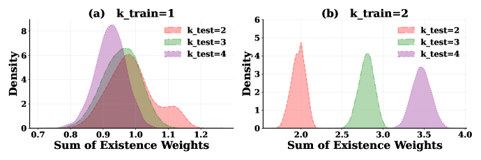
## Density Plots: Sum of Existence Weights vs. k_train and k_test ### Overview The image presents two density plots, labeled (a) and (b), visualizing the distribution of "Sum of Existence Weights" for different combinations of `k_train` and `k_test` values. Plot (a) shows data for `k_train = 1`, while plot (b) shows data for `k_train = 2`. Each plot displays density curves for `k_test` values of 2, 3, and 4, represented by different colors. ### Components/Axes * **X-axis:** "Sum of Existence Weights" - Ranges from approximately 0.7 to 1.2 in plot (a) and from approximately 2.0 to 4.0 in plot (b). * **Y-axis:** "Density" - Ranges from 0 to approximately 8 in plot (a) and from 0 to approximately 6 in plot (b). * **Legend:** Located in the top-right corner of each plot. * `k_test = 2` (Red) * `k_test = 3` (Green) * `k_test = 4` (Purple) * **Titles:** * (a) `k_train = 1` * (b) `k_train = 2` ### Detailed Analysis or Content Details **Plot (a): k_train = 1** * **k_test = 2 (Red):** The density curve is unimodal, peaking at approximately 0.85 with a density of around 7.5. The curve extends from approximately 0.7 to 1.1. * **k_test = 3 (Green):** The density curve is unimodal, peaking at approximately 0.95 with a density of around 6.5. The curve extends from approximately 0.8 to 1.2. * **k_test = 4 (Purple):** The density curve is unimodal, peaking at approximately 1.05 with a density of around 5.5. The curve extends from approximately 0.9 to 1.2. **Plot (b): k_train = 2** * **k_test = 2 (Red):** The density curve is unimodal, peaking at approximately 2.2 with a density of around 5.5. The curve extends from approximately 2.0 to 3.0. * **k_test = 3 (Green):** The density curve is unimodal, peaking at approximately 2.8 with a density of around 4.5. The curve extends from approximately 2.4 to 3.6. * **k_test = 4 (Purple):** The density curve is unimodal, peaking at approximately 3.4 with a density of around 4.0. The curve extends from approximately 3.0 to 4.0. ### Key Observations * In both plots, the density curves shift to the right as `k_test` increases. This indicates that the "Sum of Existence Weights" generally increases with higher values of `k_test`. * The peak density decreases as `k_test` increases. This suggests that the distribution becomes more spread out with higher `k_test` values. * The distributions in plot (b) (k_train = 2) are shifted to significantly higher values of "Sum of Existence Weights" compared to plot (a) (k_train = 1). * The curves are all unimodal, suggesting a single dominant value for the sum of existence weights for each k_test value. ### Interpretation The data suggests a strong relationship between `k_train`, `k_test`, and the "Sum of Existence Weights". Increasing `k_test` consistently increases the "Sum of Existence Weights", but also leads to a broader, less concentrated distribution. The substantial shift in the distributions between `k_train = 1` and `k_train = 2` indicates that `k_train` has a significant impact on the overall magnitude of the "Sum of Existence Weights". The "Sum of Existence Weights" likely represents a measure of confidence or importance assigned to certain elements within a model or system. The `k` values likely represent parameters controlling the number of elements considered or the degree of smoothing applied. The plots demonstrate how varying these parameters affects the distribution of these weights. The fact that the distributions are unimodal suggests that the system tends to converge on a single, dominant configuration for each set of parameters. The spread of the distribution indicates the degree of uncertainty or variability in this configuration. The shift to the right with increasing `k_test` could indicate that considering more elements (higher `k_test`) leads to a stronger overall signal or more significant weights.