\n
## Chart: Cumulative Distribution Function of E2E Latency
### Overview
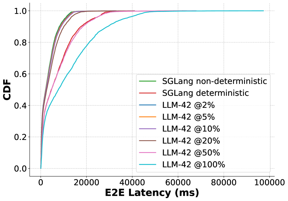
The image presents a cumulative distribution function (CDF) plot comparing the end-to-end (E2E) latency of two models, SGLang and LLM-42, under varying percentile conditions. The x-axis represents E2E Latency in milliseconds (ms), and the y-axis represents the CDF. The chart visualizes how the probability of latency being less than or equal to a given value changes for each model and percentile.
### Components/Axes
* **X-axis:** E2E Latency (ms), ranging from approximately 0 to 100000 ms.
* **Y-axis:** CDF, ranging from 0.0 to 1.0.
* **Legend:** Located in the top-right corner, listing the data series:
* SGLang non-deterministic (Teal)
* SGLang deterministic (Red)
* LLM-42 @2% (Light Blue)
* LLM-42 @5% (Orange)
* LLM-42 @10% (Light Green)
* LLM-42 @20% (Purple)
* LLM-42 @50% (Gray)
* LLM-42 @100% (Dark Gray)
### Detailed Analysis
The chart displays several CDF curves.
* **SGLang non-deterministic (Teal):** This line starts at approximately CDF 0.0 at E2E Latency 0 ms, rises rapidly to CDF 0.8 at approximately 10000 ms, and plateaus around CDF 0.95 at approximately 30000 ms, eventually reaching CDF 1.0 at around 60000 ms.
* **SGLang deterministic (Red):** This line starts at approximately CDF 0.0 at E2E Latency 0 ms, rises very steeply to CDF 0.8 at approximately 5000 ms, and plateaus around CDF 0.95 at approximately 15000 ms, reaching CDF 1.0 at around 30000 ms.
* **LLM-42 @2% (Light Blue):** This line starts at approximately CDF 0.0 at E2E Latency 0 ms, rises to CDF 0.8 at approximately 15000 ms, and plateaus around CDF 0.95 at approximately 40000 ms, reaching CDF 1.0 at around 70000 ms.
* **LLM-42 @5% (Orange):** This line starts at approximately CDF 0.0 at E2E Latency 0 ms, rises to CDF 0.8 at approximately 20000 ms, and plateaus around CDF 0.95 at approximately 50000 ms, reaching CDF 1.0 at around 80000 ms.
* **LLM-42 @10% (Light Green):** This line starts at approximately CDF 0.0 at E2E Latency 0 ms, rises to CDF 0.8 at approximately 25000 ms, and plateaus around CDF 0.95 at approximately 60000 ms, reaching CDF 1.0 at around 90000 ms.
* **LLM-42 @20% (Purple):** This line starts at approximately CDF 0.0 at E2E Latency 0 ms, rises to CDF 0.8 at approximately 30000 ms, and plateaus around CDF 0.95 at approximately 70000 ms, reaching CDF 1.0 at around 95000 ms.
* **LLM-42 @50% (Gray):** This line starts at approximately CDF 0.0 at E2E Latency 0 ms, rises to CDF 0.8 at approximately 40000 ms, and plateaus around CDF 0.95 at approximately 80000 ms, reaching CDF 1.0 at around 98000 ms.
* **LLM-42 @100% (Dark Gray):** This line starts at approximately CDF 0.0 at E2E Latency 0 ms, rises to CDF 0.8 at approximately 50000 ms, and plateaus around CDF 0.95 at approximately 90000 ms, reaching CDF 1.0 at around 100000 ms.
### Key Observations
* SGLang deterministic is consistently faster than SGLang non-deterministic, as indicated by the steeper slope and earlier plateau of its CDF curve.
* As the percentile increases for LLM-42, the CDF curve shifts to the right, indicating higher latency. Higher percentiles represent longer tail latencies.
* LLM-42 exhibits significantly higher latency than SGLang, especially at higher percentiles (e.g., 50% and 100%).
* The LLM-42 @2% curve is closest to the SGLang curves, suggesting that a small percentage of requests have relatively low latency.
### Interpretation
This chart demonstrates the trade-offs between determinism and latency in SGLang, and the overall higher latency of LLM-42. The deterministic version of SGLang provides faster and more predictable performance. The LLM-42 model shows a wider distribution of latencies, with a significant tail of slower responses, especially as the percentile increases. This suggests that while LLM-42 can sometimes respond quickly, it is more prone to experiencing longer delays compared to SGLang. The percentile values for LLM-42 indicate the latency experienced by that percentage of requests. For example, 50% of LLM-42 requests take less than approximately 40000 ms, while 100% take less than approximately 50000 ms. This data is valuable for understanding the performance characteristics of each model and making informed decisions about which model to use based on latency requirements. The chart highlights the importance of considering tail latency when evaluating model performance, particularly in applications where consistent response times are critical.