## 3D Surface Plot: Relationship Between Variables x₁ᵣ, x₂ᵣ, and True α - FE
### Overview
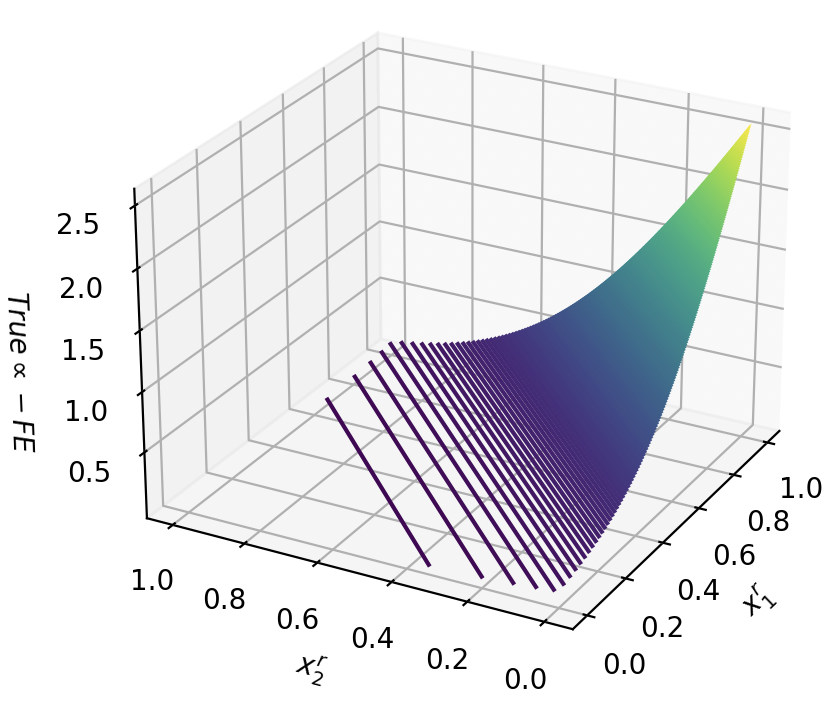
The image depicts a 3D surface plot visualizing the relationship between three variables:
- **x₁ᵣ** (horizontal axis, left-to-right)
- **x₂ᵣ** (horizontal axis, depth)
- **True α - FE** (vertical axis, z-axis)
The surface transitions from a flat region near the origin to a sharply curved, upward-sloping structure. A color gradient (purple to green) indicates increasing values of **True α - FE** with higher x₂ᵣ.
---
### Components/Axes
1. **Axes Labels**:
- **x₁ᵣ**: Ranges from 0.0 (left) to 1.0 (right).
- **x₂ᵣ**: Ranges from 0.0 (front) to 1.0 (back).
- **True α - FE**: Ranges from 0.0 (bottom) to 2.5 (top).
2. **Surface**:
- A 3D grid forms the base, with a smooth, continuous surface overlay.
- The surface is color-coded:
- **Purple**: Low values of **True α - FE** (near the origin).
- **Green**: High values of **True α - FE** (upper-right region).
3. **No Legend**:
- No explicit legend is present to confirm the meaning of the color gradient.
---
### Detailed Analysis
1. **Surface Behavior**:
- **Flat Region**: Near the origin (x₁ᵣ ≈ 0.0, x₂ᵣ ≈ 0.0), the surface is nearly flat, with **True α - FE** ≈ 0.0–0.5.
- **Curved Region**: As x₂ᵣ increases (moving backward along the plot), the surface curves upward sharply.
- At x₂ᵣ ≈ 0.8–1.0, **True α - FE** reaches ~2.5 (green region).
- **x₁ᵣ Dependency**: The surface remains relatively flat along the x₁ᵣ axis (left-to-right), suggesting weak or no dependency on x₁ᵣ.
2. **Color Gradient**:
- The transition from purple (low values) to green (high values) aligns with increasing **True α - FE** as x₂ᵣ increases.
- No explicit scale or legend is provided to quantify the color mapping.
3. **Grid Structure**:
- The 3D grid uses uniform spacing for x₁ᵣ and x₂ᵣ (0.0–1.0 in 0.2 increments).
- The z-axis (True α - FE) is labeled in 0.5 increments.
---
### Key Observations
1. **Dominant Trend**:
- **True α - FE** increases monotonically with x₂ᵣ, with minimal dependence on x₁ᵣ.
- The surface’s curvature intensifies as x₂ᵣ approaches 1.0.
2. **Anomalies**:
- No outliers or discontinuities are visible.
- The absence of a legend introduces uncertainty about the exact interpretation of the color gradient.
3. **Spatial Relationships**:
- The flat region near the origin suggests that **True α - FE** is negligible when both x₁ᵣ and x₂ᵣ are small.
- The sharp upward curve implies a nonlinear relationship between x₂ᵣ and **True α - FE**.
---
### Interpretation
1. **Mathematical Implications**:
- The plot likely represents a function **f(x₁ᵣ, x₂ᵣ) = True α - FE**, where x₂ᵣ is the primary driver of the output.
- The lack of x₁ᵣ dependency suggests the function may simplify to **f(x₂ᵣ)** in this visualization.
2. **Practical Significance**:
- If **True α - FE** represents a physical or engineering metric (e.g., stress, efficiency), the plot highlights a critical threshold: increasing x₂ᵣ beyond ~0.6 leads to a rapid rise in the metric.
- The flat region near the origin could indicate a "baseline" or "neutral" state where the metric is minimal.
3. **Uncertainties**:
- Without a legend, the exact meaning of the color gradient (e.g., whether it represents magnitude, probability, or another variable) remains ambiguous.
- The absence of numerical data points or error bars limits quantitative validation of the trends.
---
### Final Notes
This plot emphasizes the dominance of x₂ᵣ in determining **True α - FE**, with x₁ᵣ playing a negligible role. The sharp curvature and color gradient suggest a nonlinear, possibly exponential relationship between x₂ᵣ and the output. Further analysis (e.g., adding a legend, providing numerical data) would strengthen interpretability.