## Block Diagram: Signal Processing Pipeline with Homodyne Detection
### Overview
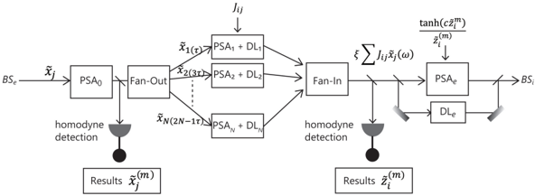
The image displays a technical block diagram of a signal processing or computational pipeline, likely within the domain of optical computing, quantum information, or advanced signal processing. The system processes an input signal `BS₀` through a series of stages involving splitting, parallel processing, combining, and detection, ultimately producing two sets of results: `Results x̃ⱼ^(m)` and `Results ẑᵢ^(m)`. The flow is primarily from left to right.
### Components/Axes
The diagram is composed of labeled blocks, arrows indicating signal/data flow, and specific operational symbols.
**Input/Output Labels:**
* **Leftmost Input:** `BS₀`
* **Rightmost Output:** `BS₁`
* **Primary Results Outputs (Bottom):**
* Left: `Results x̃ⱼ^(m)`
* Right: `Results ẑᵢ^(m)`
**Processing Blocks (in flow order):**
1. **PSA₀**: First processing block after input.
2. **Fan-Out**: Splits the signal into multiple parallel paths.
3. **Parallel Processing Branches (N branches):** Each branch contains a block labeled `PSAₙ + DLₙ` (where n = 1, 2, ..., N). The diagram explicitly shows:
* `PSA₁ + DL₁`
* `PSA₂ + DL₂`
* `PSAₙ + DLₙ` (indicating the nth branch)
* The signals entering these branches are labeled `x̃₁(1/2)`, `x̃₂(1/2)`, ..., `x̃ₙ(2N-1/2N)`.
4. **Fan-In**: Combines the outputs from the parallel branches.
5. **PSAₑ**: A final processing block after the Fan-In and a summation operation.
6. **Homodyne Detection Units:** Two units are present.
* One taps the signal after `PSA₀` and before `Fan-Out`, feeding into `Results x̃ⱼ^(m)`.
* Another taps the signal after `Fan-In` and before `PSAₑ`, feeding into `Results ẑᵢ^(m)`.
**Mathematical/Operational Symbols:**
* **Jᵢⱼ**: An input or parameter feeding into the parallel processing stage.
* **Σ (Summation):** A summation operation `Σ Jᵢⱼ x̃ⱼ(ω)` is applied to the signal after `Fan-In`.
* **tanh(c ẑᵢ^(m)):** A hyperbolic tangent function applied to a signal `ẑᵢ^(m)`, which appears to be an input or feedback to the `PSAₑ` block.
* **Arrows:** Indicate the direction of signal flow throughout the system.
* **Homodyne Detection Symbol:** Represented by a semicircle with a line, connected to a black circle (detector).
### Detailed Analysis
**Signal Flow and Processing:**
1. The input signal `BS₀` enters `PSA₀`.
2. The output of `PSA₀` splits. One path goes to a homodyne detector for immediate measurement (`Results x̃ⱼ^(m)`). The main path goes to `Fan-Out`.
3. `Fan-Out` creates N parallel copies of the signal, labeled `x̃₁(1/2)` through `x̃ₙ(2N-1/2N)`.
4. Each parallel copy is processed by a dedicated block `PSAₙ + DLₙ`. These blocks also receive an external input or parameter `Jᵢⱼ`.
5. The outputs of all N parallel branches are combined by the `Fan-In` block.
6. The combined signal from `Fan-In` is then subjected to a summation operation: `Σ Jᵢⱼ x̃ⱼ(ω)`.
7. The signal after summation splits. One path goes to a second homodyne detector for measurement (`Results ẑᵢ^(m)`). The main path proceeds to the `PSAₑ` block.
8. The `PSAₑ` block also receives an input derived from `tanh(c ẑᵢ^(m))`, suggesting a feedback or nonlinear transformation based on the second measurement result.
9. The final output of the system is `BS₁`.
**Component Isolation:**
* **Header/Left Section:** Input (`BS₀`), initial processing (`PSA₀`), and first measurement point.
* **Main Central Section:** The parallel processing core consisting of `Fan-Out`, N branches of `PSAₙ + DLₙ`, and `Fan-In`.
* **Footer/Right Section:** Post-combination processing (`Σ`, `PSAₑ`), second measurement point, and final output (`BS₁`).
### Key Observations
1. **Parallel Architecture:** The system's core is a parallelized structure (`Fan-Out` to `Fan-In`), suggesting it performs multiple operations simultaneously on split versions of the signal.
2. **Dual Measurement Points:** There are two distinct homodyne detection stages, measuring the signal at different points in the pipeline (`x̃ⱼ^(m)` early, `ẑᵢ^(m)` later).
3. **Feedback/Nonlinearity:** The presence of `tanh(c ẑᵢ^(m))` as an input to the final `PSAₑ` block indicates a nonlinear element or a feedback loop where a later measurement influences prior processing.
4. **Parameterized Processing:** The parallel branches are not identical; they are indexed (`PSA₁ + DL₁` to `PSAₙ + DLₙ`) and receive a parameter `Jᵢⱼ`, implying weighted or differentiated processing across channels.
5. **Notation:** The use of tildes (`~`) and subscripts/superscripts (`ⱼ`, `ᵢ`, `^(m)`) is consistent with mathematical notation for signals, indices, and iteration steps common in signal processing and machine learning literature.
### Interpretation
This diagram represents a sophisticated signal processing pipeline, potentially for tasks like signal estimation, filtering, or machine learning inference in a physical (e.g., optical) system. The structure suggests an algorithm that:
1. **Encodes/Preprocesses:** `PSA₀` likely performs an initial transformation (e.g., Phase-Sensitive Amplification, suggested by "PSA").
2. **Parallelizes:** The `Fan-Out` / `Fan-In` structure with weighted branches (`Jᵢⱼ`) resembles a neural network layer or a bank of filters, where the input is processed by multiple units in parallel.
3. **Measures and Adapts:** The two homodyne detection stages provide measurement outcomes. The second measurement `ẑᵢ^(m)` is transformed (`tanh`) and fed back into the final processing stage (`PSAₑ`), indicating an adaptive or iterative refinement process. This could be part of a feedback control loop or an algorithm that uses intermediate results to adjust subsequent processing.
4. **Models Physical Processes:** The specific blocks (`PSA`, `DL` for Delay Line?, `homodyne detection`) strongly point to an implementation in optical or quantum systems, where such components are fundamental. The diagram abstracts a complex physical process into a computational flowchart.
The overall purpose appears to be the transformation of an input signal (`BS₀`) into an output (`BS₁`) through a combination of parallel linear processing (the branches) and nonlinear feedback (the `tanh` path), with key internal states being measured. It could model a physical neural network, a quantum measurement circuit, or an advanced adaptive filter.