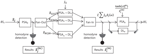
## Diagram: Quantum Reservoir Computing Architecture ### Overview The image depicts a quantum reservoir computing architecture. It shows the flow of quantum information through a series of processing stages, including phase-sensitive amplifiers (PSAs), delay lines (DLs), fan-out and fan-in operations, and homodyne detection. The diagram illustrates how input signals are processed and transformed within the quantum reservoir to produce output results. ### Components/Axes * **Input:** BS_e (Beam Splitter input) * **Output:** BS_i (Beam Splitter output) * **Processing Units:** * PSA₀: Phase-Sensitive Amplifier 0 * Fan-Out: Signal distribution unit * PSA₁ + DL₁: Phase-Sensitive Amplifier 1 + Delay Line 1 * PSA₂ + DL₂: Phase-Sensitive Amplifier 2 + Delay Line 2 * PSA_N + DL_N: Phase-Sensitive Amplifier N + Delay Line N * Fan-In: Signal aggregation unit * PSA_e: Phase-Sensitive Amplifier e * DL_e: Delay Line e * **Signals:** * x̃_j: Input signal * x̃₁(τ): Signal after Fan-Out, first branch * x̃₂(3τ): Signal after Fan-Out, second branch * x̃_N(2N-1τ): Signal after Fan-Out, Nth branch * ξ ∑ J_ijx̃_j(ω): Summation of weighted signals * tanh(c z̃_i^(m)) / z̃_i^(m): Non-linear transformation * **Detection:** * Homodyne detection (two instances) * **Results:** * Results x̃_j^(m): Output from the first homodyne detection * Results z̃_i^(m): Output from the second homodyne detection * **Weights:** * J_ij: Weights applied to the signals ### Detailed Analysis 1. **Input Stage:** The input signal x̃_j enters the system through a beam splitter (BS_e) and is processed by the first phase-sensitive amplifier (PSA₀). 2. **Fan-Out:** The signal is then distributed by the Fan-Out unit into N branches. The signals in these branches are denoted as x̃₁(τ), x̃₂(3τ), ..., x̃_N(2N-1τ). 3. **Processing Branches:** Each branch consists of a phase-sensitive amplifier (PSA_i) and a delay line (DL_i), where i ranges from 1 to N. 4. **Fan-In:** The signals from all N branches are aggregated by the Fan-In unit. The aggregated signal is represented as ξ ∑ J_ijx̃_j(ω), where J_ij represents the weights applied to the signals. 5. **Output Stage:** The aggregated signal is then processed by another phase-sensitive amplifier (PSA_e) and a delay line (DL_e). A non-linear transformation, tanh(c z̃_i^(m)) / z̃_i^(m), is applied before PSA_e. The final output signal exits through a beam splitter (BS_i). 6. **Homodyne Detection:** Homodyne detection is performed after PSA₀ and after the Fan-In unit. The results of these detections are x̃_j^(m) and z̃_i^(m), respectively. ### Key Observations * The architecture uses multiple phase-sensitive amplifiers and delay lines to process the input signal. * The Fan-Out and Fan-In units distribute and aggregate the signals, respectively. * Homodyne detection is used to measure the quantum states at different stages of the processing. * The non-linear transformation tanh(c z̃_i^(m)) / z̃_i^(m) introduces non-linearity into the system. ### Interpretation The diagram illustrates a quantum reservoir computing architecture, which leverages the complex dynamics of a quantum system to perform computational tasks. The input signal is processed through a series of non-linear transformations and feedback loops within the reservoir, allowing the system to learn and adapt to different input patterns. The homodyne detection provides a means to measure the quantum states and extract the computational results. The architecture is designed to exploit the unique properties of quantum mechanics, such as superposition and entanglement, to achieve computational advantages over classical systems. The weights J_ij are crucial for training the reservoir to perform specific tasks. The delay lines introduce temporal dynamics, which are essential for processing time-dependent signals.