## Diagram: Probabilistic Graphical Model (Sub-model)
### Overview
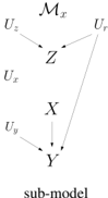
The image displays a directed acyclic graph (DAG), specifically a probabilistic graphical model or causal diagram. It illustrates the hypothesized relationships between several variables, denoted by single letters and symbols, and exogenous factors or noise terms, denoted by `U` with subscripts. The diagram is labeled at the bottom as a "sub-model," suggesting it is a component of a larger system.
### Components/Axes
The diagram consists of nodes (variables) and directed edges (arrows indicating influence or conditional dependence).
**Nodes (Variables):**
* **M_ε**: A top-level node, likely representing a model parameter, mechanism, or latent variable.
* **Z**: A central node, potentially a latent variable or mediator.
* **X**: A node positioned below Z.
* **Y**: The bottom-most node, often representing the outcome variable in such models.
* **U₂, U₃, U₄, U₅, U₆, U₇**: A set of exogenous variables, noise terms, or unobserved confounders. Each is connected to one of the main variables (Z, X, Y).
**Edges (Directed Arrows):**
* From **M_ε** to **Z**.
* From **Z** to **X**.
* From **Z** to **Y**.
* From **X** to **Y**.
* From **U₂** to **Z**.
* From **U₃** to **Z**.
* From **U₄** to **X**.
* From **U₅** to **X**.
* From **U₆** to **Y**.
* From **U₇** to **Y**.
**Text Label:**
* The phrase **"sub-model"** is centered at the very bottom of the diagram.
### Detailed Analysis
The structure defines a specific set of conditional independence assumptions.
1. **Variable Hierarchy and Flow:** The primary causal or generative flow appears to be: `M_ε → Z → {X, Y}` and `X → Y`. This creates a path `Z → X → Y` and a direct path `Z → Y`.
2. **Exogenous Inputs:** Each of the endogenous variables (Z, X, Y) is influenced by two distinct exogenous factors (`U` terms). This is a common way to model independent noise or unobserved influences affecting each variable.
* **Z** is influenced by `U₂` and `U₃`.
* **X** is influenced by `U₄` and `U₅`.
* **Y** is influenced by `U₆` and `U₇`.
3. **Spatial Layout:** The diagram is arranged vertically to imply a temporal or causal sequence. `M_ε` is at the top (most upstream), `Z` is in the upper-middle, `X` is in the lower-middle, and `Y` is at the bottom (most downstream). The `U` nodes are placed to the left of their respective target variables.
### Key Observations
* **No Cycles:** The graph is acyclic, which is a requirement for standard Bayesian networks and many causal inference frameworks.
* **Collider at Y:** Node `Y` is a collider, as it has two direct parents: `Z` and `X`. In causal inference, conditioning on a collider (like Y) can induce spurious associations between its parents (Z and X).
* **Mediation:** Variable `X` acts as a mediator for part of the effect of `Z` on `Y` (the path `Z → X → Y`), while also allowing a direct effect (`Z → Y`).
* **Symmetry in Noise:** The model assigns exactly two independent exogenous inputs to each of the three main variables (Z, X, Y), suggesting a deliberate and symmetric modeling choice for uncertainty or external influence.
### Interpretation
This diagram formally represents a hypothesis about the data-generating process for variables X, Y, and Z, under the influence of a higher-level parameter M_ε.
* **What it Suggests:** The model posits that `Z` is a key latent factor influenced by `M_ε`. `Z` then directly affects both `X` and `Y`. Furthermore, `X` has a direct effect on `Y`. Therefore, the total effect of `Z` on `Y` is the sum of a direct effect and an indirect effect mediated through `X`. The `U` terms account for all other variation in each variable.
* **Relationships:** It encodes a specific set of conditional independence statements. For example, `X` and `Y` are not independent given `Z` (because of the direct `Z→Y` edge and the `Z→X→Y` path). However, `X` and the exogenous terms `U₂/U₃` affecting `Z` are independent.
* **Purpose as a "Sub-model":** This structure is likely a modular component. `M_ε` could be a parameter shared across multiple such sub-models, or `Z` could be a latent variable whose distribution is defined elsewhere in a larger model. The diagram is a precise tool for communication in fields like statistics, machine learning, econometrics, or epidemiology, allowing researchers to debate and test causal assumptions.