## Network Sparsification and Degree Distribution
### Overview
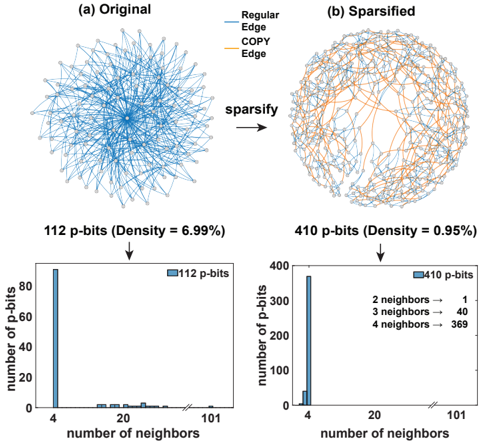
The image presents a comparison between an original network and its sparsified version, along with their respective degree distributions. The image is divided into two columns, (a) Original and (b) Sparsified. Each column contains a network diagram and a histogram showing the number of p-bits versus the number of neighbors. The sparsification process reduces the density of the network, which is reflected in the change in the degree distribution.
### Components/Axes
**Top Row: Network Diagrams**
* **(a) Original:** A dense network diagram with nodes connected by "Regular Edge" (blue lines).
* **(b) Sparsified:** A less dense network diagram with nodes connected by "Regular Edge" (blue lines) and "COPY Edge" (orange lines).
* **Legend (Top-Right):**
* Regular Edge: Blue line
* COPY Edge: Orange line
* **Process Indicator:** An arrow labeled "sparsify" points from the original network to the sparsified network.
**Bottom Row: Histograms (Degree Distributions)**
* **X-axis (both histograms):** "number of neighbors" with tick marks at 4, 20, and 101. A break in the x-axis indicates a discontinuity in the scale.
* **Y-axis (both histograms):** "number of p-bits" ranging from 0 to 80 for the original network and 0 to 400 for the sparsified network.
* **Histogram Bars:** Blue bars representing the frequency of each number of neighbors.
* **Titles above Histograms:**
* Left: "112 p-bits (Density = 6.99%)"
* Right: "410 p-bits (Density = 0.95%)"
* **Legends within Histograms:**
* Left: "112 p-bits"
* Right: "410 p-bits"
* **Additional Text (Right Histogram):**
* 2 neighbors → 1
* 3 neighbors → 40
* 4 neighbors → 369
### Detailed Analysis or ### Content Details
**Network Diagrams:**
* **(a) Original:** The network appears highly connected, with many blue edges linking the nodes.
* **(b) Sparsified:** The network has fewer blue edges and the introduction of orange edges. The overall connectivity is reduced.
**Histograms:**
* **(a) Original:**
* The histogram is heavily skewed towards a small number of neighbors.
* The bar at 4 neighbors reaches approximately 80 p-bits.
* The bars for higher numbers of neighbors are very small, close to zero.
* **(b) Sparsified:**
* The histogram is also skewed towards a small number of neighbors, but the distribution is different from the original.
* The bar at 4 neighbors reaches approximately 370 p-bits.
* The text indicates specific values: 2 neighbors (1 p-bit), 3 neighbors (40 p-bits), and 4 neighbors (369 p-bits).
### Key Observations
* The sparsification process significantly reduces the density of the network (from 6.99% to 0.95%).
* The number of p-bits increases from 112 to 410 after sparsification.
* The degree distribution shifts after sparsification, with a higher concentration of nodes having a small number of neighbors (specifically 4 neighbors).
### Interpretation
The image illustrates the effect of sparsification on a network and its degree distribution. Sparsification, while reducing the overall density of connections, can lead to a redistribution of node degrees. The increase in p-bits after sparsification suggests that the process involves adding new nodes or connections, even as it removes others. The degree distributions show that both the original and sparsified networks are dominated by nodes with a small number of neighbors, but the sparsified network has a much higher concentration of nodes with 4 neighbors. This could indicate that the sparsification algorithm preferentially creates or preserves connections that result in nodes having a degree of 4. The "COPY Edge" likely represents edges that were created during the sparsification process, potentially duplicating or re-wiring existing connections.