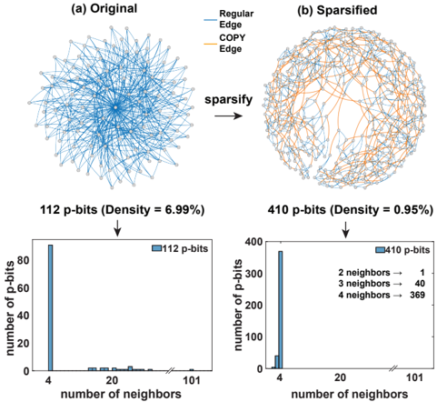
## Network Sparsification and P-bit Distribution Analysis ### Overview This image presents a comparative analysis of a network before and after a sparsification process, along with the corresponding distributions of "p-bits" based on the number of neighbors. It consists of two network diagrams illustrating the structural change, and two bar charts (histograms) showing the distribution of p-bits for each state. ### Components/Axes **Top Section: Network Diagrams** * **Title (Overall):** The top section is divided into two sub-sections: * **(a) Original**: Located on the top-left. * **(b) Sparsified**: Located on the top-right. * **Transformation:** An arrow labeled "sparsify" points from the "Original" network to the "Sparsified" network, indicating a process of reducing network density. * **Legend (Top-right, common to both networks):** * **Regular Edge**: Represented by a blue line. * **COPY Edge**: Represented by an orange line. * **Network (a) Original:** * Composed of numerous small, light grey circular nodes interconnected by a dense web of blue lines (Regular Edges). The network appears highly connected and centrally concentrated. * **Network (b) Sparsified:** * Composed of the same type of small, light grey circular nodes. The network is visibly less dense than the original. It features both blue lines (Regular Edges) and orange lines (COPY Edges), with orange edges being prominent and forming a more structured, perhaps ring-like, pattern around the periphery, while blue edges are also present but less numerous than in the original. **Middle Section: Summary Statistics** * **Below (a) Original:** "112 p-bits (Density = 6.99%)" * **Below (b) Sparsified:** "410 p-bits (Density = 0.95%)" * **Transformation Arrows:** Downward arrows connect these summary statistics to their respective bar charts below. **Bottom Section: Bar Charts (Histograms)** * **Common Y-axis Label (Left and Right):** "number of p-bits" * Scale: Ranges from 0 to 80 (left chart) and 0 to 400 (right chart) in increments of 20 or 100, respectively. * **Common X-axis Label (Left and Right):** "number of neighbors" * Scale: Ranges from 0 to 101, with major ticks at 4, 20, and 101. A break in the X-axis (indicated by `//`) is present between approximately 35 and 100, suggesting a non-linear or truncated scale for higher neighbor counts. ### Detailed Analysis **Network Diagrams:** * **Original Network (a):** Shows a very dense graph where most connections are "Regular Edges" (blue). The nodes are arranged in a roughly circular fashion, but the high density of edges makes individual connections difficult to discern. * **Sparsified Network (b):** This network is significantly less dense. The "sparsify" process has resulted in a network where "COPY Edges" (orange) are clearly visible and form a substantial part of the remaining connections, often appearing to connect nodes in a more structured, perhaps local, manner compared to the original's overall density. "Regular Edges" (blue) are still present but are fewer and less dominant than in the original. **Summary Statistics:** * The "Original" state has **112 p-bits** and a network **Density of 6.99%**. * The "Sparsified" state has **410 p-bits** and a significantly lower network **Density of 0.95%**. This indicates that the sparsification process drastically reduced the network density while increasing the total number of "p-bits". **Bar Chart (Left) - Original (112 p-bits):** * **Legend:** A blue rectangle labeled "112 p-bits" is located in the top-right of the chart. * **Trend:** The distribution is highly skewed towards a low number of neighbors. * **Data Points:** * At "number of neighbors" = 4, there is a very tall bar, approximately 88-89 "number of p-bits". * At "number of neighbors" = ~19-20, there is a very small bar, approximately 2-3 "number of p-bits". * At "number of neighbors" = ~26-27, there is another very small bar, approximately 1-2 "number of p-bits". * At "number of neighbors" = ~31-32, there is another very small bar, approximately 1-2 "number of p-bits". * Beyond these points, up to 101, no significant bars are visible. **Bar Chart (Right) - Sparsified (410 p-bits):** * **Legend:** A blue rectangle labeled "410 p-bits" is located in the top-right of the chart. * **Trend:** The distribution is extremely concentrated at very low numbers of neighbors, specifically 2, 3, and 4. * **Data Points (from embedded text):** * **2 neighbors → 1** (A very small bar at x=2, height 1) * **3 neighbors → 40** (A bar at x=3, height 40) * **4 neighbors → 369** (A very tall bar at x=4, height 369) * The sum of these p-bits (1 + 40 + 369 = 410) matches the total "410 p-bits" indicated in the legend and the summary text above. ### Key Observations * **Sparsification Effect:** The "sparsify" process dramatically reduces network density (from 6.99% to 0.95%). * **P-bit Increase:** Counter-intuitively, the total number of "p-bits" increases significantly after sparsification (from 112 to 410). This suggests "p-bits" might represent something other than just edges, perhaps specific structural motifs or information units that become more prominent or are defined differently in a sparser context. * **Edge Type Change:** The sparsified network introduces "COPY Edges" (orange), which were not explicitly present or distinguished in the original network's legend. This implies a reclassification or creation of new edge types during sparsification. * **Neighbor Distribution Shift:** Both original and sparsified networks show a highly skewed distribution of p-bits towards a low number of neighbors. * In the original network, the vast majority of p-bits (around 89 out of 112) are associated with 4 neighbors. * In the sparsified network, the distribution becomes even more concentrated and precise, with almost all p-bits (410 out of 410) having 2, 3, or 4 neighbors, with the largest group (369 p-bits) still having 4 neighbors. The distribution is much "cleaner" and less spread out in the sparsified state. ### Interpretation The image illustrates a process of network sparsification that, rather than simply removing edges, appears to transform the network in a way that increases a metric called "p-bits" while drastically reducing the overall network density. This suggests that "p-bits" are not a direct count of edges or nodes, but rather a measure of specific structural elements or information content that might be enhanced or revealed through the sparsification process. The introduction of "COPY Edges" in the sparsified network is crucial. It implies that the sparsification is not just about removing "Regular Edges" but potentially identifying and highlighting certain connections as "COPY Edges," which might be critical for maintaining specific network properties or information flow in a sparser representation. The visual prominence of orange "COPY Edges" in the sparsified network supports this. The change in the "number of p-bits" distribution is also highly informative. While both networks show a preference for p-bits having a low number of neighbors, the sparsified network exhibits an extremely sharp and well-defined distribution, almost exclusively at 2, 3, and 4 neighbors. This suggests that the sparsification process effectively filters or reorganizes the network such that the "p-bits" that remain or are generated conform to very specific local connectivity patterns (i.e., having 2, 3, or 4 neighbors). The increase in total p-bits from 112 to 410, despite the massive reduction in density, implies that the sparsification process might be extracting or defining more "meaningful" or "efficient" p-bits from the original dense structure. This could be interpreted as a form of feature extraction or simplification where the essential information (represented by p-bits) is amplified and clarified, even as the raw connectivity (density) is reduced. The original network, with its higher density and more spread-out p-bit distribution, might contain redundant or less critical connections that are pruned or re-evaluated during sparsification.