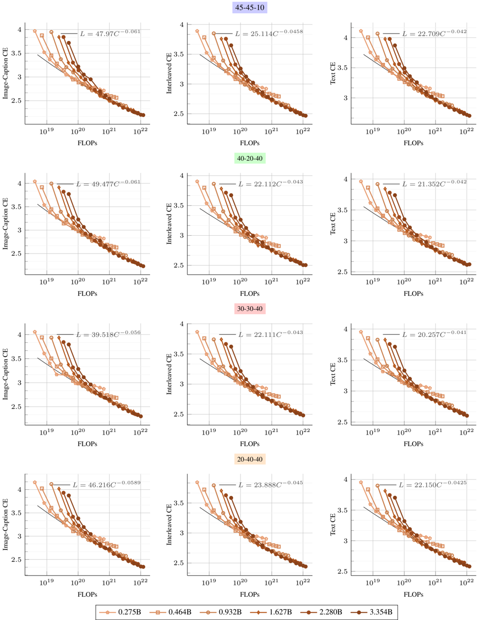
## Chart: Performance vs. Compute for Different Data Mixes ### Overview The image presents a series of scatter plots showing the relationship between performance (CE - Cross Entropy) and compute (FLOPS - Floating Point Operations Per Second) for different data mixes. Each plot represents a different data mix configuration (45-45-10, 40-20-40, 30-30-40, 20-40-40), and within each plot, different lines represent different model sizes. The plots are arranged in a 2x3 grid. ### Components/Axes * **X-axis (FLOPS):** Represents the computational cost in Floating Point Operations Per Second. The scale is logarithmic, ranging from approximately 10^19 to 10^22. * **Y-axis (Image-Caption CE, Interleaved CE, Text CE):** Represents the cross-entropy loss, a measure of performance. The scale ranges from 2.5 to 4.0. The Y-axis label varies depending on the column: "Image-Caption CE" for the first column, "Interleaved CE" for the second column, and "Text CE" for the third column. * **Data Series:** Each line on the plot represents a different model size, indicated by the legend at the bottom. The model sizes are 0.275B, 0.464B, 0.932B, 1.627B, 2.280B, and 3.354B. * **Titles:** Each plot has a title indicating the data mix configuration (e.g., 45-45-10, 40-20-40, etc.). * **Trend Lines:** Each plot includes a black trend line, with an equation of the form L = aC^(-b), where L is the loss, C is the compute, and a and b are constants. ### Detailed Analysis **Plot 1: 45-45-10, Image-Caption CE** * Trend: As FLOPS increase, Image-Caption CE decreases. * Equation: L = 47.97C^(-0.061) * Data Points: * 0.275B (lightest color): Starts at approximately (10^19, 4.0), ends around (10^22, 2.4) * 0.464B: Starts at approximately (10^19, 3.8), ends around (10^22, 2.3) * 0.932B: Starts at approximately (10^19, 3.6), ends around (10^22, 2.3) * 1.627B: Starts at approximately (10^19, 3.4), ends around (10^22, 2.2) * 2.280B: Starts at approximately (10^19, 3.2), ends around (10^22, 2.2) * 3.354B (darkest color): Starts at approximately (10^19, 3.0), ends around (10^22, 2.1) **Plot 2: 45-45-10, Interleaved CE** * Trend: As FLOPS increase, Interleaved CE decreases. * Equation: L = 25.114C^(-0.0458) * Data Points: * 0.275B: Starts at approximately (10^19, 4.0), ends around (10^22, 2.5) * 0.464B: Starts at approximately (10^19, 3.7), ends around (10^22, 2.4) * 0.932B: Starts at approximately (10^19, 3.5), ends around (10^22, 2.4) * 1.627B: Starts at approximately (10^19, 3.3), ends around (10^22, 2.3) * 2.280B: Starts at approximately (10^19, 3.1), ends around (10^22, 2.3) * 3.354B: Starts at approximately (10^19, 2.9), ends around (10^22, 2.2) **Plot 3: 45-45-10, Text CE** * Trend: As FLOPS increase, Text CE decreases. * Equation: L = 22.709C^(-0.042) * Data Points: * 0.275B: Starts at approximately (10^19, 4.0), ends around (10^22, 2.5) * 0.464B: Starts at approximately (10^19, 3.7), ends around (10^22, 2.4) * 0.932B: Starts at approximately (10^19, 3.5), ends around (10^22, 2.4) * 1.627B: Starts at approximately (10^19, 3.3), ends around (10^22, 2.3) * 2.280B: Starts at approximately (10^19, 3.1), ends around (10^22, 2.3) * 3.354B: Starts at approximately (10^19, 2.9), ends around (10^22, 2.2) **Plot 4: 40-20-40, Image-Caption CE** * Trend: As FLOPS increase, Image-Caption CE decreases. * Equation: L = 49.477C^(-0.061) * Data Points: * 0.275B: Starts at approximately (10^19, 4.0), ends around (10^22, 2.4) * 0.464B: Starts at approximately (10^19, 3.8), ends around (10^22, 2.3) * 0.932B: Starts at approximately (10^19, 3.6), ends around (10^22, 2.3) * 1.627B: Starts at approximately (10^19, 3.4), ends around (10^22, 2.2) * 2.280B: Starts at approximately (10^19, 3.2), ends around (10^22, 2.2) * 3.354B: Starts at approximately (10^19, 3.0), ends around (10^22, 2.1) **Plot 5: 40-20-40, Interleaved CE** * Trend: As FLOPS increase, Interleaved CE decreases. * Equation: L = 22.112C^(-0.043) * Data Points: * 0.275B: Starts at approximately (10^19, 4.0), ends around (10^22, 2.5) * 0.464B: Starts at approximately (10^19, 3.7), ends around (10^22, 2.4) * 0.932B: Starts at approximately (10^19, 3.5), ends around (10^22, 2.4) * 1.627B: Starts at approximately (10^19, 3.3), ends around (10^22, 2.3) * 2.280B: Starts at approximately (10^19, 3.1), ends around (10^22, 2.3) * 3.354B: Starts at approximately (10^19, 2.9), ends around (10^22, 2.2) **Plot 6: 40-20-40, Text CE** * Trend: As FLOPS increase, Text CE decreases. * Equation: L = 21.352C^(-0.042) * Data Points: * 0.275B: Starts at approximately (10^19, 4.0), ends around (10^22, 2.5) * 0.464B: Starts at approximately (10^19, 3.7), ends around (10^22, 2.4) * 0.932B: Starts at approximately (10^19, 3.5), ends around (10^22, 2.4) * 1.627B: Starts at approximately (10^19, 3.3), ends around (10^22, 2.3) * 2.280B: Starts at approximately (10^19, 3.1), ends around (10^22, 2.3) * 3.354B: Starts at approximately (10^19, 2.9), ends around (10^22, 2.2) **Plot 7: 30-30-40, Image-Caption CE** * Trend: As FLOPS increase, Image-Caption CE decreases. * Equation: L = 39.518C^(-0.056) * Data Points: * 0.275B: Starts at approximately (10^19, 4.0), ends around (10^22, 2.4) * 0.464B: Starts at approximately (10^19, 3.8), ends around (10^22, 2.3) * 0.932B: Starts at approximately (10^19, 3.6), ends around (10^22, 2.3) * 1.627B: Starts at approximately (10^19, 3.4), ends around (10^22, 2.2) * 2.280B: Starts at approximately (10^19, 3.2), ends around (10^22, 2.2) * 3.354B: Starts at approximately (10^19, 3.0), ends around (10^22, 2.1) **Plot 8: 30-30-40, Interleaved CE** * Trend: As FLOPS increase, Interleaved CE decreases. * Equation: L = 22.111C^(-0.043) * Data Points: * 0.275B: Starts at approximately (10^19, 4.0), ends around (10^22, 2.5) * 0.464B: Starts at approximately (10^19, 3.7), ends around (10^22, 2.4) * 0.932B: Starts at approximately (10^19, 3.5), ends around (10^22, 2.4) * 1.627B: Starts at approximately (10^19, 3.3), ends around (10^22, 2.3) * 2.280B: Starts at approximately (10^19, 3.1), ends around (10^22, 2.3) * 3.354B: Starts at approximately (10^19, 2.9), ends around (10^22, 2.2) **Plot 9: 30-30-40, Text CE** * Trend: As FLOPS increase, Text CE decreases. * Equation: L = 20.257C^(-0.041) * Data Points: * 0.275B: Starts at approximately (10^19, 4.0), ends around (10^22, 2.5) * 0.464B: Starts at approximately (10^19, 3.7), ends around (10^22, 2.4) * 0.932B: Starts at approximately (10^19, 3.5), ends around (10^22, 2.4) * 1.627B: Starts at approximately (10^19, 3.3), ends around (10^22, 2.3) * 2.280B: Starts at approximately (10^19, 3.1), ends around (10^22, 2.3) * 3.354B: Starts at approximately (10^19, 2.9), ends around (10^22, 2.2) **Plot 10: 20-40-40, Image-Caption CE** * Trend: As FLOPS increase, Image-Caption CE decreases. * Equation: L = 46.216C^(-0.0589) * Data Points: * 0.275B: Starts at approximately (10^19, 4.0), ends around (10^22, 2.4) * 0.464B: Starts at approximately (10^19, 3.8), ends around (10^22, 2.3) * 0.932B: Starts at approximately (10^19, 3.6), ends around (10^22, 2.3) * 1.627B: Starts at approximately (10^19, 3.4), ends around (10^22, 2.2) * 2.280B: Starts at approximately (10^19, 3.2), ends around (10^22, 2.2) * 3.354B: Starts at approximately (10^19, 3.0), ends around (10^22, 2.1) **Plot 11: 20-40-40, Interleaved CE** * Trend: As FLOPS increase, Interleaved CE decreases. * Equation: L = 23.888C^(-0.045) * Data Points: * 0.275B: Starts at approximately (10^19, 4.0), ends around (10^22, 2.5) * 0.464B: Starts at approximately (10^19, 3.7), ends around (10^22, 2.4) * 0.932B: Starts at approximately (10^19, 3.5), ends around (10^22, 2.4) * 1.627B: Starts at approximately (10^19, 3.3), ends around (10^22, 2.3) * 2.280B: Starts at approximately (10^19, 3.1), ends around (10^22, 2.3) * 3.354B: Starts at approximately (10^19, 2.9), ends around (10^22, 2.2) **Plot 12: 20-40-40, Text CE** * Trend: As FLOPS increase, Text CE decreases. * Equation: L = 22.150C^(-0.0425) * Data Points: * 0.275B: Starts at approximately (10^19, 4.0), ends around (10^22, 2.5) * 0.464B: Starts at approximately (10^19, 3.7), ends around (10^22, 2.4) * 0.932B: Starts at approximately (10^19, 3.5), ends around (10^22, 2.4) * 1.627B: Starts at approximately (10^19, 3.3), ends around (10^22, 2.3) * 2.280B: Starts at approximately (10^19, 3.1), ends around (10^22, 2.3) * 3.354B: Starts at approximately (10^19, 2.9), ends around (10^22, 2.2) ### Key Observations * **Inverse Relationship:** There is a clear inverse relationship between FLOPS and CE. As the computational cost increases, the cross-entropy loss decreases, indicating improved performance. * **Model Size Impact:** Larger models (higher number of parameters) generally achieve lower CE (better performance) for a given amount of compute. * **Data Mix Impact:** The data mix configuration influences the overall performance. The equations for the trend lines vary across different data mixes, suggesting that some mixes are more efficient than others. * **Similar Trends:** The trends are qualitatively similar across different data mixes and CE types (Image-Caption, Interleaved, Text). ### Interpretation The data suggests that increasing computational resources (FLOPS) and model size leads to improved performance, as measured by cross-entropy loss. The specific data mix used during training also plays a role in the final performance, as evidenced by the different trend line equations. The consistent trends across different CE types indicate that the observed relationships are robust and not specific to a particular task. The equations provided allow for a quantitative comparison of the efficiency of different data mixes. The plots demonstrate the trade-off between compute, model size, and performance, which is a crucial consideration in machine learning model development.