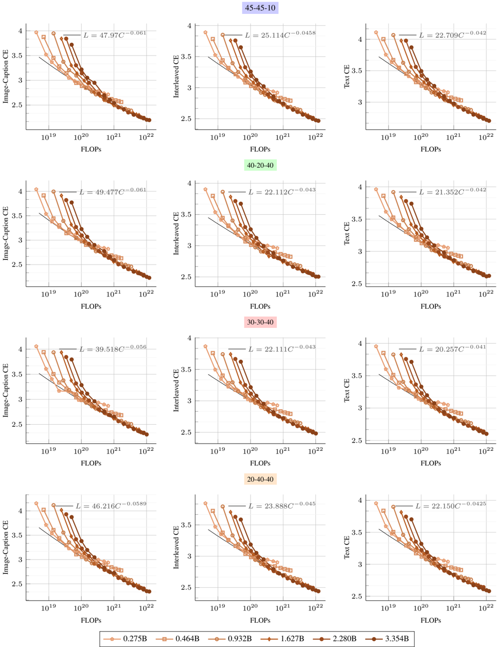
## Scatter Plot Grid: Scaling Laws for Multimodal Models ### Overview The image displays a 4x3 grid of scatter plots illustrating the relationship between computational cost (FLOPs) and model performance (Cross-Entropy loss) for different multimodal model configurations. The plots are organized into four rows, each representing a distinct model architecture ratio (e.g., 45-45-10), and three columns representing different evaluation tasks: Image-Caption CE, Interleaved CE, and Text CE. Each plot contains multiple data series corresponding to different model parameter sizes, with fitted power-law scaling curves. ### Components/Axes * **Grid Structure:** 4 rows x 3 columns. * **Row Labels (Top of each row):** * Row 1: `45-45-10` (light blue background) * Row 2: `40-20-40` (light green background) * Row 3: `30-30-40` (light pink background) * Row 4: `20-40-40` (light orange background) * **Column Labels (Y-axis titles):** * Column 1: `Image-Caption CE` * Column 2: `Interleaved CE` * Column 3: `Text CE` * **X-axis (All plots):** `FLOPs` (logarithmic scale, ranging from approximately `10^19` to `10^22`). * **Y-axis (All plots):** Cross-Entropy (CE) loss (linear scale, ranging from approximately `2.5` to `4.0`). * **Legend (Bottom center of entire image):** A horizontal legend mapping model parameter sizes to colors and markers. * `0.275B`: Lightest orange, circle marker. * `0.464B`: Light orange, square marker. * `0.932B`: Medium orange, diamond marker. * `1.627B`: Darker orange, upward-pointing triangle marker. * `2.280B`: Dark brown, downward-pointing triangle marker. * `3.354B`: Darkest brown, hexagon marker. * **Fitted Equations:** Each plot contains a text annotation in the top-right corner showing a fitted power-law equation of the form `L = a * C^(-b)`, where `L` is loss and `C` is FLOPs. ### Detailed Analysis **Data Series & Trends:** For every plot, the data series (points) show a clear downward trend: as FLOPs increase (moving right on the x-axis), the Cross-Entropy loss decreases (moving down on the y-axis). The points for larger models (darker colors) are consistently positioned to the right (higher FLOPs) and lower (lower loss) than points for smaller models (lighter colors), forming a consistent scaling curve. **Extracted Fitted Equations (L = a * C^(-b)):** * **Row 1 (45-45-10):** * Image-Caption CE: `L = 47.97C^(-0.061)` * Interleaved CE: `L = 25.114C^(-0.0458)` * Text CE: `L = 22.709C^(-0.042)` * **Row 2 (40-20-40):** * Image-Caption CE: `L = 49.477C^(-0.061)` * Interleaved CE: `L = 22.112C^(-0.043)` * Text CE: `L = 21.352C^(-0.042)` * **Row 3 (30-30-40):** * Image-Caption CE: `L = 39.518C^(-0.056)` * Interleaved CE: `L = 22.111C^(-0.043)` * Text CE: `L = 20.257C^(-0.041)` * **Row 4 (20-40-40):** * Image-Caption CE: `L = 46.216C^(-0.0589)` * Interleaved CE: `L = 23.888C^(-0.045)` * Text CE: `L = 22.150C^(-0.0425)` **Spatial Grounding & Verification:** The legend is positioned at the bottom center of the entire figure. Within each individual plot, the fitted equation is consistently placed in the top-right corner. The color/marker mapping from the legend is applied consistently across all 12 plots. For example, the darkest brown hexagon (`3.354B`) is always the rightmost and lowest point in each series, confirming it represents the largest model with the best performance. ### Key Observations 1. **Consistent Scaling Law:** All 12 plots demonstrate a strong power-law relationship between compute (FLOPs) and loss. The negative exponent (`-b`) in every fitted equation confirms that loss decreases predictably as compute increases. 2. **Task-Dependent Scaling:** The scaling exponent (`b`) and coefficient (`a`) vary by task and model configuration. * **Image-Caption CE** tasks consistently show the steepest scaling (largest `b` values, ~0.056 to 0.061), indicating loss improves most rapidly with added compute for this task. * **Text CE** tasks show the shallowest scaling (smallest `b` values, ~0.041 to 0.0425), suggesting diminishing returns from additional compute on pure text tasks. * **Interleaved CE** tasks fall in between. 3. **Configuration Impact:** The model architecture ratio (e.g., 45-45-10 vs. 20-40-40) influences the absolute loss values (coefficient `a`) but has a less dramatic effect on the scaling exponent (`b`), especially for Text and Interleaved tasks where exponents are very similar across rows. 4. **Data Density:** The plots contain a high density of data points, especially in the mid-to-high FLOP range (`10^20` to `10^22`), providing robust evidence for the fitted curves. ### Interpretation This image presents empirical evidence for **scaling laws in multimodal AI models**. The core finding is that model performance, measured by cross-entropy loss on image-captioning, interleaved image-text, and pure text tasks, improves predictably as a power-law function of the computational resources (FLOPs) used for training. The data suggests that: * **Investment in compute yields predictable returns:** The tight fit of the data points to the power-law curves implies that one can forecast the performance of a larger model trained with more FLOPs based on the performance of smaller models. * **Task nature dictates scaling efficiency:** The steeper slope for Image-Caption CE indicates that multimodal understanding (aligning images and text) benefits more dramatically from increased scale than pure text modeling does. This could imply that the "bottleneck" for image-captioning performance is more directly alleviated by model size and data, whereas text modeling may be approaching a plateau or is limited by other factors. * **Architecture matters for absolute performance, less for scaling rate:** While changing the model's internal ratio (the row labels) shifts the entire curve up or down (changing `a`), it doesn't drastically alter the fundamental rate of improvement with scale (`b`). This suggests the scaling *phenomenon* is robust, but careful architecture design is still crucial for achieving the best possible loss at any given compute budget. The absence of significant outliers indicates the experiments were well-controlled. The primary "anomaly" is the notably different scaling exponent for the Image-Caption task, which is the most significant finding and highlights the unique scaling properties of multimodal versus unimodal learning.