## State Transition Diagram: Permutation Sorting Example
### Overview
The image displays a technical diagram illustrating two examples of state transitions from an initial permutation of numbers to a sorted goal state. It is a simple, black-and-white schematic likely used to explain concepts in algorithms, sorting, or problem-solving.
### Components/Axes
The diagram is organized into two horizontal rows, each representing a separate example labeled **P1** and **P2**.
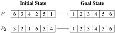
* **Top Labels:** The columns are labeled **"Initial State"** (left) and **"Goal State"** (right).
* **Row Labels:** The rows are labeled **P1** (top row) and **P2** (bottom row).
* **Visual Elements:** Each state is represented by a series of adjacent rectangular boxes, each containing a single digit. A right-pointing arrow (`→`) connects the "Initial State" to the "Goal State" for each row.
### Detailed Analysis
**Row P1:**
* **Initial State (Left):** A sequence of six boxes containing the numbers: `6`, `3`, `4`, `2`, `5`, `1`.
* **Goal State (Right):** A sequence of six boxes containing the numbers in ascending order: `1`, `2`, `3`, `4`, `5`, `6`.
* **Transformation:** An arrow indicates the transition from the unsorted initial sequence to the sorted goal sequence.
**Row P2:**
* **Initial State (Left):** A sequence of six boxes containing the numbers: `3`, `2`, `1`, `6`, `5`, `4`.
* **Goal State (Right):** A sequence of six boxes containing the numbers in ascending order: `1`, `2`, `3`, `4`, `5`, `6`.
* **Transformation:** An arrow indicates the transition from the unsorted initial sequence to the sorted goal sequence.
### Key Observations
1. **Identical Goal:** Both examples, P1 and P2, share the exact same **Goal State**: the sequence `[1, 2, 3, 4, 5, 6]`.
2. **Different Initial States:** The **Initial States** are different permutations of the same set of numbers {1, 2, 3, 4, 5, 6}.
* P1's initial state is `[6, 3, 4, 2, 5, 1]`.
* P2's initial state is `[3, 2, 1, 6, 5, 4]`.
3. **Visual Trend:** The diagram visually demonstrates a process of **ordering** or **sorting**. The trend for both rows is from a disordered, non-sequential arrangement on the left to a perfectly ordered, sequential arrangement on the right.
4. **Spatial Layout:** The layout is clean and comparative. The parallel structure (two rows, two columns) allows for easy side-by-side comparison of the two different starting points leading to the same end result.
### Interpretation
This diagram serves as a clear, abstract representation of a **sorting problem** or a **state-space search** problem. It demonstrates that multiple, distinct initial configurations (permutations) can be transformed into a single, desired goal configuration (the sorted list).
* **What it suggests:** The core concept is that of a **function** or **algorithm** (implied by the arrow) that takes an unordered input and produces an ordered output. The specific algorithm is not shown, only its input-output pairs.
* **Relationship between elements:** The "Initial State" and "Goal State" are directly linked by a transformation process. The two rows (P1, P2) are independent examples that reinforce the universality of the goal state regardless of the starting point.
* **Notable patterns:** The most significant pattern is the **convergence** of different initial states to a single goal state. This is a fundamental property of deterministic sorting algorithms. There are no outliers; both examples perfectly follow the rule of transforming a permutation into its sorted form.
* **Underlying purpose:** This type of diagram is commonly used in computer science education to introduce sorting algorithms (like Bubble Sort, Insertion Sort), in mathematics to discuss permutations, or in AI to illustrate problem states in a search space. It visually answers the question: "What does it mean to sort these numbers?" by showing concrete before-and-after examples.