# Technical Document Extraction: Anomaly Detection Workflow
## 1. Normal Period Data
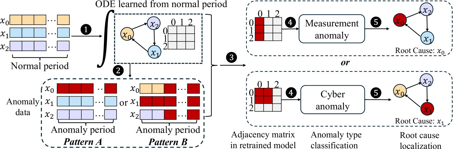
- **Structure**:
- Three time-series variables (`x0`, `x1`, `x2`)
- Colored blocks represent data points:
- `x0`: Yellow
- `x1`: Blue
- `x2`: Purple
- Legend placement: Left side of diagram
- Spatial grounding:
- Normal period data: `[x=0, y=0]` to `[x=2, y=2]`
## 2. Anomaly Detection Process
### 2.1 ODE Learning from Normal Period
- **Flow**:
- Arrow `1` connects normal period to ODE learning block
- Process outputs:
- Learned variables: `x0`, `x1`, `x2`
- Adjacency matrix (3x3) with values `0`, `1`, `2`
- **Spatial grounding**:
- ODE learning block: `[x=1, y=0]`
### 2.2 Anomaly Period Analysis
- **Data Segmentation**:
- Two anomaly patterns:
- **Pattern A**:
- `x0`: Red (anomaly)
- `x1`: Blue (normal)
- `x2`: Purple (normal)
- **Pattern B**:
- `x0`: Yellow (normal)
- `x1`: Red (anomaly)
- `x2`: Purple (normal)
- Color legend mapping:
- Red: Anomaly
- Blue/Purple: Normal
- Yellow: Normal (original normal period)
## 3. Adjacency Matrix Analysis
- **Matrix Structure**:
- 3x3 grid with values `0`, `1`, `2`
- Red blocks highlight changes from normal period
- **Spatial grounding**:
- Adjacency matrix: `[x=1, y=1]`
## 4. Anomaly Type Classification
### 4.1 Measurement Anomaly
- **Root Cause**:
- `x0` (red block)
- Spatial grounding: `[x=2, y=0]`
- **Flow**:
- Adjacency matrix → Measurement anomaly → Root cause localization
### 4.2 Cyber Anomaly
- **Root Cause**:
- `x1` (red block)
- Spatial grounding: `[x=2, y=1]`
- **Flow**:
- Adjacency matrix → Cyber anomaly → Root cause localization
## 5. Key Technical Components
1. **Color-Coded Legend**:
- Yellow: Normal `x0`
- Blue: Normal `x1`
- Purple: Normal `x2`
- Red: Anomaly
- Spatial reference: `[x=0, y=0]` to `[x=2, y=2]`
2. **Process Flow**:
- Normal period data → ODE learning → Adjacency matrix → Anomaly classification → Root cause localization
3. **Critical Data Points**:
- Measurement anomaly root cause: `x0` (red)
- Cyber anomaly root cause: `x1` (red)
- Adjacency matrix values: `0`, `1`, `2` with red highlights
## 6. Trend Verification
- **Normal Period**:
- Consistent color patterns (no red blocks)
- **Anomaly Periods**:
- Pattern A: Red block in `x0` column
- Pattern B: Red block in `x1` column
- Visual trend: Vertical red blocks indicate anomaly type
## 7. Component Isolation
### 7.1 Header
- Title: "ODE learned from normal period"
- Spatial: `[x=1, y=0]`
### 7.2 Main Chart
- Adjacency matrix analysis
- Anomaly type classification
### 7.3 Footer
- Root cause localization (x0/x1)
- Spatial: `[x=2, y=0]` to `[x=2, y=1]`
## 8. Data Table Reconstruction
| Variable | Normal Color | Anomaly Color | Anomaly Type | Root Cause |
|----------|--------------|---------------|-------------------|------------|
| x0 | Yellow | Red | Measurement | x0 |
| x1 | Blue | Red | Cyber | x1 |
| x2 | Purple | Purple | Normal | - |
## 9. Spatial Grounding Summary
- Normal period: `[x=0, y=0]` to `[x=2, y=2]`
- ODE learning: `[x=1, y=0]`
- Adjacency matrix: `[x=1, y=1]`
- Anomaly classification: `[x=2, y=0]` (Measurement), `[x=2, y=1]` (Cyber)