# Technical Document Extraction: Visualizing Efficiency in RAN Topology Learning
## 1. Document Header
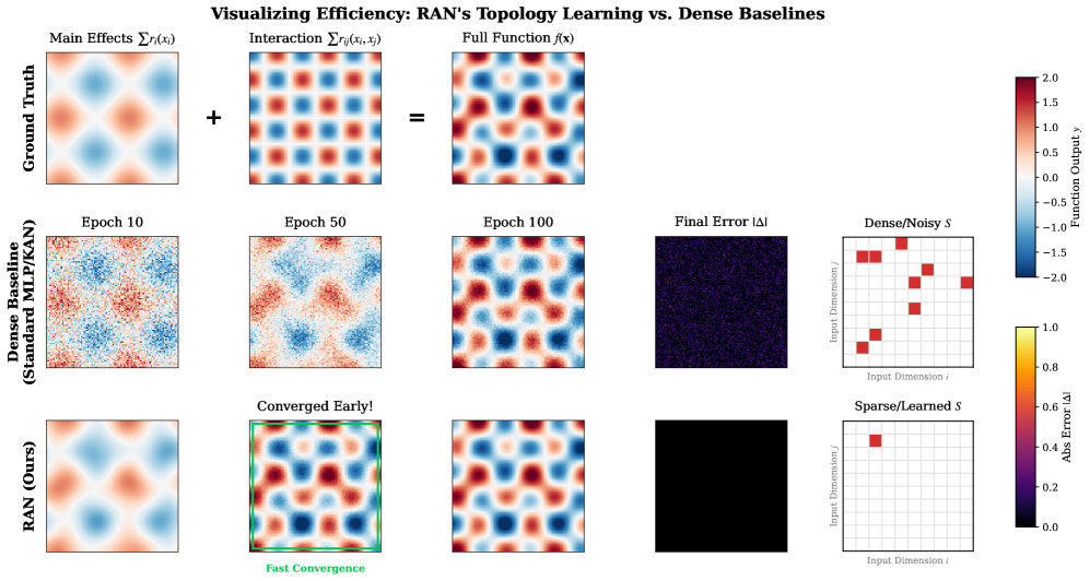
* **Title:** Visualizing Efficiency: RAN's Topology Learning vs. Dense Baselines
* **Primary Subject:** Comparison of function approximation and convergence speed between a standard Dense Baseline (MLP/KAN) and a proposed RAN (Ours) model.
---
## 2. Component Isolation & Layout
The image is organized into a grid structure with three primary rows and five functional columns, plus two vertical color scales on the right.
### Row 1: Ground Truth (The Target)
This row defines the mathematical function the models are attempting to learn.
* **Column 1: Main Effects $\sum r_i(x_i)$**
* *Visual:* A low-frequency heatmap showing a soft diamond pattern of alternating red (positive) and blue (negative) values.
* **Column 2: Interaction $\sum r_{ij}(x_i, x_j)$**
* *Visual:* A high-frequency checkerboard pattern of red and blue, indicating complex local interactions.
* *Operator:* A large **"+"** sign sits between Column 1 and Column 2.
* **Column 3: Full Function $f(\mathbf{x})$**
* *Visual:* The summation of the first two plots. It shows a complex, multi-modal landscape.
* *Operator:* An **"="** sign sits between Column 2 and Column 3.
### Row 2: Dense Baseline (Standard MLP/KAN)
Shows the progression of a standard dense model over training epochs.
* **Column 1: Epoch 10** - Visual is very noisy; the underlying pattern is barely discernible.
* **Column 2: Epoch 50** - The pattern begins to emerge but remains grainy and low-resolution.
* **Column 3: Epoch 100** - The model has captured the general shape of the Full Function but retains visible noise/artifacts.
* **Column 4: Final Error $|\Delta|$** - A dark purple heatmap with significant speckled noise, indicating residual error across the domain.
* **Column 5: Dense/Noisy $S$** - A $10 \times 10$ grid representing input dimensions $i$ (x-axis) and $j$ (y-axis). It contains approximately 10 scattered red squares, indicating a non-optimized or noisy selection of feature interactions.
### Row 3: RAN (Ours)
Shows the progression of the proposed Relational Additive Network.
* **Column 1: Epoch 10** - Visual is smooth and already closely resembles the "Main Effects" of the Ground Truth.
* **Column 2: Converged Early!** - This plot is highlighted with a **bright green border**. It shows a high-fidelity reconstruction of the Full Function. Below the plot is the text: **"Fast Convergence"** in green.
* **Column 3: Epoch 100** - A clean, smooth reconstruction identical to the Ground Truth Full Function.
* **Column 4: Final Error $|\Delta|$** - A solid black square. Per the error scale, black represents $0.0$ error, indicating near-perfect convergence.
* **Column 5: Sparse/Learned $S$** - A $10 \times 10$ grid representing input dimensions $i$ and $j$. It contains only **one** red square at coordinates (approx. $i=3, j=8$), indicating the model successfully identified the specific sparse interaction required.
---
## 3. Data Scales (Legends)
Located at the far right of the image.
### Scale 1: Function Output $y$ (Top Right)
* **Type:** Diverging Color Map (Blue to White to Red)
* **Range:** $[-2.0, 2.0]$
* **Markers:** $2.0, 1.5, 1.0, 0.5, 0.0, -0.5, -1.0, -1.5, -2.0$
* **Interpretation:** Red indicates high positive values; Blue indicates high negative values; White is neutral (0).
### Scale 2: Abs Error $|\Delta|$ (Bottom Right)
* **Type:** Sequential Color Map (Black to Purple to Orange to Yellow)
* **Range:** $[0.0, 1.0]$
* **Markers:** $1.0, 0.8, 0.6, 0.4, 0.2, 0.0$
* **Interpretation:** Black indicates zero error; Yellow indicates maximum error ($1.0$).
---
## 4. Key Trends and Technical Observations
1. **Convergence Speed:** The **RAN** model achieves a high-fidelity reconstruction by "Epoch 50" (labeled as Converged Early), whereas the **Dense Baseline** is still highly noisy at "Epoch 100".
2. **Accuracy:** The "Final Error" plot for RAN is solid black (Error $\approx 0$), while the Dense Baseline shows a "Final Error" that is dark purple/speckled (Error $\approx 0.2 - 0.3$ visually).
3. **Structural Sparsity:** The "Sparse/Learned $S$" grid demonstrates that RAN identifies the exact interaction needed (one red block), while the Dense Baseline utilizes a "Dense/Noisy" set of interactions (multiple red blocks), leading to overfitting or inefficiency.
4. **Signal Reconstruction:** RAN captures the "Main Effects" smoothly by Epoch 10, suggesting an inductive bias that prioritizes additive components before refining interactions.