## Line Chart: Runtime for solving OneMinMax
### Overview
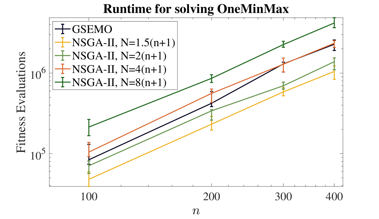
The image is a line chart comparing the computational runtime (measured in fitness evaluations) of five different algorithms or algorithm configurations for solving the "OneMinMax" problem. The runtime is plotted against the problem size, denoted by `n`. All data series show a clear increasing trend, with runtime growing as `n` increases. The chart uses a logarithmic scale for the y-axis.
### Components/Axes
* **Title:** "Runtime for solving OneMinMax" (centered at the top).
* **X-Axis:**
* **Label:** `n` (centered below the axis).
* **Scale:** Linear scale with major tick marks and labels at `100`, `200`, `300`, and `400`.
* **Y-Axis:**
* **Label:** "Fitness Evaluations" (rotated 90 degrees, left side).
* **Scale:** Logarithmic scale (base 10). Major tick marks and labels are at `10^5` and `10^6`. Minor tick marks are present between these major values.
* **Legend:** Located in the top-left corner of the plot area. It contains five entries, each with a colored line segment, a marker, and a text label.
1. **Label:** `GSEMO` | **Color/Marker:** Dark blue line with a plus (`+`) marker.
2. **Label:** `NSGA-II, N=1.5(n+1)` | **Color/Marker:** Yellow-orange line with a plus (`+`) marker.
3. **Label:** `NSGA-II, N=2(n+1)` | **Color/Marker:** Light green line with a plus (`+`) marker.
4. **Label:** `NSGA-II, N=4(n+1)` | **Color/Marker:** Orange-red line with a plus (`+`) marker.
5. **Label:** `NSGA-II, N=8(n+1)` | **Color/Marker:** Dark green line with a plus (`+`) marker.
* **Data Series:** Five lines, each with error bars (vertical lines with caps) at the data points for `n=100, 200, 300, 400`.
### Detailed Analysis
The following table reconstructs the approximate data points for each algorithm. Values are estimated from the logarithmic y-axis. The trend for all series is a roughly linear increase on this log-linear plot, indicating an exponential relationship between `n` and the number of fitness evaluations.
| Algorithm (Legend Label) | Color | Approx. Fitness Evaluations at n=100 | Approx. Fitness Evaluations at n=200 | Approx. Fitness Evaluations at n=300 | Approx. Fitness Evaluations at n=400 | Visual Trend Description |
| :--- | :--- | :--- | :--- | :--- | :--- | :--- |
| **GSEMO** | Dark Blue | ~9 x 10^4 | ~4 x 10^5 | ~1.2 x 10^6 | ~2.5 x 10^6 | Steep, consistent upward slope. |
| **NSGA-II, N=1.5(n+1)** | Yellow-Orange | ~5 x 10^4 | ~2 x 10^5 | ~5 x 10^5 | ~1 x 10^6 | Shallowest slope among the series. Lowest runtime at all points. |
| **NSGA-II, N=2(n+1)** | Light Green | ~7 x 10^4 | ~3 x 10^5 | ~7 x 10^5 | ~1.2 x 10^6 | Slope is steeper than N=1.5 but less steep than others. |
| **NSGA-II, N=4(n+1)** | Orange-Red | ~1 x 10^5 | ~6 x 10^5 | ~1.2 x 10^6 | ~2.5 x 10^6 | Very steep slope, similar to GSEMO. Intersects with GSEMO line near n=300. |
| **NSGA-II, N=8(n+1)** | Dark Green | ~2 x 10^5 | ~9 x 10^5 | ~2 x 10^6 | ~4 x 10^6 | Steepest slope overall. Highest runtime at all points. |
**Error Bars:** All data points have vertical error bars, indicating variability in the measured runtime. The length of the error bars appears relatively consistent across the series for a given `n`, though they are more pronounced on the logarithmic scale at higher values.
### Key Observations
1. **Clear Hierarchy:** There is a consistent performance hierarchy across all problem sizes (`n`). From fastest (lowest evaluations) to slowest: `NSGA-II, N=1.5(n+1)` < `NSGA-II, N=2(n+1)` < `GSEMO` ≈ `NSGA-II, N=4(n+1)` < `NSGA-II, N=8(n+1)`.
2. **Impact of N:** For the NSGA-II algorithm, increasing the population size parameter `N` (from 1.5(n+1) to 8(n+1)) results in a significant increase in runtime (fitness evaluations).
3. **GSEMO vs. NSGA-II:** The GSEMO algorithm's performance is comparable to NSGA-II with `N=4(n+1)`. Their lines are very close and intersect around `n=300`.
4. **Scaling Behavior:** All algorithms exhibit what appears to be exponential scaling with respect to `n`, as indicated by the roughly straight lines on the log-linear plot. The slope of the line (the exponent) varies between algorithms.
### Interpretation
This chart demonstrates the computational cost scaling of different evolutionary algorithms on the OneMinMax benchmark problem. The key insight is the trade-off between algorithm configuration and runtime.
* **Population Size Matters:** For NSGA-II, a larger population size (`N`) leads to dramatically higher computational cost. The `N=8(n+1)` variant is approximately an order of magnitude more expensive than the `N=1.5(n+1)` variant at `n=400`. This suggests that while larger populations might offer other benefits (like solution quality or diversity), they come at a steep runtime penalty for this problem.
* **Algorithm Comparison:** GSEMO, a multi-objective evolutionary algorithm based on a steady-state genetic algorithm and a archive, shows a runtime profile similar to a moderately configured NSGA-II (`N=4(n+1)`). This provides a point of reference for comparing different algorithmic paradigms.
* **Practical Implication:** For large problem sizes (`n`), the choice of algorithm and its parameters has a massive impact on feasibility. Using the most efficient configuration shown (`NSGA-II, N=1.5(n+1)`) could mean solving a problem with `n=400` in roughly 1 million evaluations, whereas the least efficient (`NSGA-II, N=8(n+1)`) would require around 4 million evaluations—a fourfold increase in computational resources.
* **Underlying Pattern:** The linear trend on the log plot suggests the runtime `R` can be modeled as `R ≈ a * b^n`, where `b` is a base greater than 1. The different slopes indicate different values of `b` for each algorithm configuration, quantifying their relative scalability.