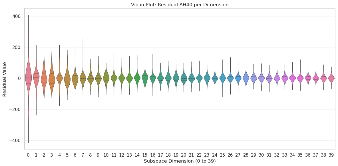
## Violin Plot: Residual ΔH40 per Dimension ### Overview The image is a violin plot showing the distribution of residual values for different subspace dimensions, ranging from 0 to 39. The plot visualizes the probability density of the residual values for each dimension, with the width of the "violin" indicating the frequency of values at that level. The color of the violins transitions from pink/red on the left to purple/pink on the right. ### Components/Axes * **Title:** Violin Plot: Residual ΔH40 per Dimension * **X-axis:** Subspace Dimension (0 to 39). The axis is marked with integers from 0 to 39. * **Y-axis:** Residual Value. The axis is marked with -400, -200, 0, 200, and 400. * **Violin Plots:** Each violin plot represents the distribution of residual values for a specific subspace dimension. The width of the violin indicates the density of data points at a given residual value. A dashed horizontal line is present in the center of each violin. * **Colors:** The violins transition in color from left to right, starting with pink/red, moving through orange, brown, green, blue, and ending with purple/pink. ### Detailed Analysis The violin plots show the distribution of residual values for each subspace dimension. * **Dimensions 0-10:** The violins are wider and have a larger range of residual values, indicating greater variability. The color ranges from pink to brown. * **Dimensions 11-25:** The violins become narrower, indicating a smaller range of residual values and less variability. The color ranges from green to blue. * **Dimensions 26-39:** The violins remain relatively narrow, with a consistent range of residual values. The color ranges from blue to purple/pink. Specifically: * Dimension 0: The violin plot is centered around 0, with a wide distribution ranging from approximately -300 to +300. * Dimension 1: The violin plot is centered around 0, with a wide distribution ranging from approximately -250 to +250. * Dimension 5: The violin plot is centered around 0, with a wide distribution ranging from approximately -200 to +200. * Dimension 10: The violin plot is centered around 0, with a wide distribution ranging from approximately -150 to +150. * Dimension 15: The violin plot is centered around 0, with a narrow distribution ranging from approximately -100 to +100. * Dimension 20: The violin plot is centered around 0, with a narrow distribution ranging from approximately -100 to +100. * Dimension 25: The violin plot is centered around 0, with a narrow distribution ranging from approximately -100 to +100. * Dimension 30: The violin plot is centered around 0, with a narrow distribution ranging from approximately -100 to +100. * Dimension 35: The violin plot is centered around 0, with a narrow distribution ranging from approximately -100 to +100. * Dimension 39: The violin plot is centered around 0, with a narrow distribution ranging from approximately -100 to +100. ### Key Observations * The variability of residual values decreases as the subspace dimension increases. * The distribution of residual values appears to be centered around zero for all dimensions. * The color gradient provides a visual cue for the change in distribution across dimensions. ### Interpretation The violin plot suggests that the residual values are more variable for lower subspace dimensions and become more consistent as the dimension increases. This could indicate that the model's performance stabilizes or becomes more predictable with higher-dimensional subspaces. The concentration of residual values around zero for all dimensions suggests that the model is generally unbiased, but the decreasing variability indicates that the model's precision improves with higher dimensions. The color gradient visually reinforces this trend, making it easier to discern the change in distribution across dimensions.