## Chart: Violin Plot - Residual ΔH40 per Dimension
### Overview
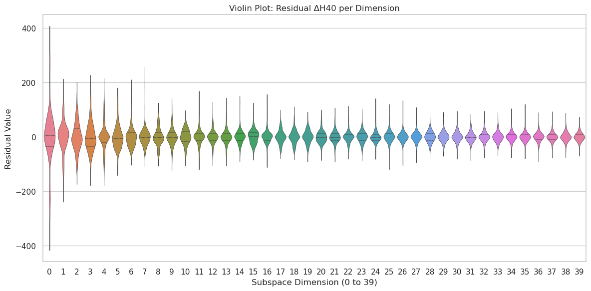
The image displays a violin plot visualizing the distribution of residual ΔH40 values across 40 dimensions (indexed from 0 to 39). The plot shows the range and density of the residuals for each dimension, providing insight into how well the model fits the data in each subspace.
### Components/Axes
* **Title:** "Violin Plot: Residual ΔH40 per Dimension" - positioned at the top-center of the image.
* **X-axis:** "Subspace Dimension (0 to 39)" - located at the bottom of the chart, with tick marks representing each dimension from 0 to 39.
* **Y-axis:** "Residual Value" - located on the left side of the chart, ranging from approximately -400 to 400.
* **Violin Plots:** 40 individual violin plots, one for each dimension. Each violin plot represents the distribution of residual values for that dimension.
* **Whiskers:** Extending from each violin plot, indicating the range of the data.
### Detailed Analysis
The violin plots are colored in a rainbow gradient, transitioning from red (dimension 0) to violet (dimension 39). Each violin plot shows the distribution of residual values.
Here's a breakdown of the approximate residual value ranges for each dimension, based on visual inspection of the violin plots:
* **Dimensions 0-4 (Red to Orange):** These dimensions exhibit a wider distribution of residuals, with values extending to approximately -300 and +250. The median residual value appears to be around 50-100.
* **Dimensions 5-10 (Orange to Yellow):** The distribution narrows slightly, with residuals ranging from approximately -250 to +200. The median residual value is around 0-50.
* **Dimensions 11-17 (Yellow to Green):** The distributions continue to narrow, with residuals ranging from approximately -200 to +150. The median residual value is around -20 to 20.
* **Dimensions 18-25 (Green to Cyan):** The distributions are relatively consistent, with residuals ranging from approximately -150 to +100. The median residual value is around -10 to 10.
* **Dimensions 26-32 (Cyan to Blue):** The distributions remain similar to the previous range, with residuals ranging from approximately -100 to +80. The median residual value is around -10 to 10.
* **Dimensions 33-39 (Blue to Violet):** The distributions are the narrowest, with residuals ranging from approximately -80 to +80. The median residual value is around 0.
The width of each violin plot indicates the density of the residual values. Wider sections represent higher densities, while narrower sections represent lower densities. The whiskers extend to approximately the 5th and 95th percentiles of the data.
### Key Observations
* The distribution of residuals appears to be centered around zero for most dimensions, suggesting a good model fit.
* The initial dimensions (0-4) exhibit the widest distribution of residuals, indicating a potentially poorer model fit in those subspaces.
* The distribution of residuals becomes narrower as the dimension number increases, suggesting that the model fits the data better in higher dimensions.
* There are no obvious outliers in any of the violin plots.
### Interpretation
The violin plot suggests that the model's performance varies across different dimensions. The initial dimensions have larger residuals, indicating that the model struggles to capture the underlying patterns in those subspaces. As the dimension number increases, the residuals become smaller, suggesting that the model is better able to fit the data in higher dimensions. This could be due to several factors, such as the importance of different features in different dimensions, or the presence of non-linear relationships that the model is unable to capture.
The narrowing of the distributions as the dimension number increases could also indicate that the higher dimensions are less informative or more correlated with each other. This could lead to a more stable and predictable model fit.
Overall, the violin plot provides a valuable visualization of the model's performance across different dimensions, allowing for a more nuanced understanding of its strengths and weaknesses. The data suggests that feature selection or dimensionality reduction techniques could be used to improve the model's performance by focusing on the most informative dimensions.