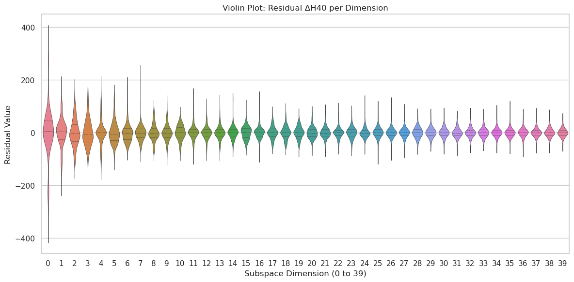
## Violin Plot: Residual ΔH40 per Dimension ### Overview The image displays a violin plot visualizing the distribution of residual ΔH40 values across 40 subspace dimensions (0–39). Each dimension is represented by a colored violin plot, with colors transitioning from red (dimension 0) to blue (dimension 39). The y-axis represents residual values ranging from -400 to 400, while the x-axis lists subspace dimensions. The plot includes three key lines per violin: a central line (median), a thick line (75th percentile), and a thin line (25th percentile). ### Components/Axes - **Title**: "Violin Plot: Residual ΔH40 per Dimension" (top center). - **X-axis**: Labeled "Subspace Dimension (0 to 39)", with ticks at every integer from 0 to 39. - **Y-axis**: Labeled "Residual Value", scaled from -400 to 400 in increments of 200. - **Legend**: A gradient bar at the bottom right, transitioning from red (dimension 0) to blue (dimension 39), with no explicit labels. - **Violin Elements**: Each violin contains: - A central horizontal line (median). - A thick horizontal line (75th percentile). - A thin horizontal line (25th percentile). - A shaded area representing the distribution density. ### Detailed Analysis - **Dimension 0 (Red)**: - Widest distribution, spanning from -400 to 400. - Central line at ~0, thick line at ~20, thin line at ~10. - High density near 0, with outliers extending to ±400. - **Dimensions 1–9 (Red-Orange Gradient)**: - Gradual narrowing of spread; peaks shift slightly below 0. - Central lines remain near 0, thick lines decrease from ~20 to ~10. - Thin lines stabilize around ~5. - **Dimensions 10–19 (Green Gradient)**: - Further narrowing; peaks cluster tightly around 0. - Central lines at ~0, thick lines at ~5, thin lines at ~2. - Reduced outliers compared to earlier dimensions. - **Dimensions 20–39 (Blue Gradient)**: - Minimal spread; peaks almost perfectly centered at 0. - Central lines at ~0, thick lines at ~2, thin lines at ~1. - Uniform density with no visible outliers. ### Key Observations 1. **Spread Reduction**: Residual variability decreases significantly as subspace dimension increases, with dimensions 20–39 showing near-zero spread. 2. **Peak Shift**: Early dimensions (0–9) exhibit peaks slightly below 0, while later dimensions (10–39) cluster tightly at 0. 3. **Color Gradient**: Red-to-blue transition correlates with decreasing residual magnitude, suggesting a systematic trend in ΔH40 values. 4. **Line Consistency**: The 75th percentile (thick line) consistently lies above the 25th percentile (thin line), confirming positive skewness in early dimensions. ### Interpretation The plot demonstrates that residual ΔH40 values become increasingly concentrated around 0 as subspace dimension increases, indicating improved stability or convergence in higher dimensions. The color gradient (red to blue) likely reflects residual magnitude, with red representing larger residuals (dimension 0) and blue smaller residuals (dimension 39). The narrowing spread suggests that higher dimensions capture more consistent or predictable patterns, while early dimensions exhibit greater variability, possibly due to noise or less informative features. The central line at 0 across most dimensions implies that the median residual value is consistently near zero, though early dimensions show larger deviations. This could indicate a trade-off between dimensionality and residual error in the analyzed system.