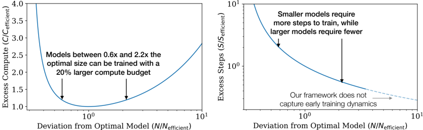
## Chart Type: Comparative Line Graphs ### Overview The image presents two line graphs side-by-side, comparing the "Deviation from Optimal Model (N/N_efficient)" on the x-axis against "Excess Compute (C/C_efficient)" on the left and "Excess Steps (S/S_efficient)" on the right. Both x-axes are on a log scale. The left graph shows the relationship between model size deviation and excess compute, while the right graph shows the relationship between model size deviation and excess steps. ### Components/Axes **Left Graph:** * **Y-axis:** "Excess Compute (C/C_efficient)". Scale ranges from 1.0 to 4.0, with tick marks at 1.0, 1.5, 2.0, 2.5, 3.0, 3.5, and 4.0. * **X-axis:** "Deviation from Optimal Model (N/N_efficient)". Logarithmic scale, ranging from 10^-1 to 10^1. Tick marks at 10^-1, 10^0, and 10^1. * **Line:** A single blue line representing the relationship between deviation from optimal model size and excess compute. * **Annotation:** "Models between 0.6x and 2.2x the optimal size can be trained with a 20% larger compute budget." Two downward-pointing arrows indicate the approximate range on the x-axis. **Right Graph:** * **Y-axis:** "Excess Steps (S/S_efficient)". Logarithmic scale, ranging from 10^0 to 10^1. Tick marks at 10^0 and 10^1. * **X-axis:** "Deviation from Optimal Model (N/N_efficient)". Logarithmic scale, ranging from 10^-1 to 10^1. Tick marks at 10^-1, 10^0, and 10^1. * **Line:** A blue line representing the relationship between deviation from optimal model size and excess steps. The line transitions to a dashed light-gray line towards the right side of the graph. * **Annotation 1:** "Smaller models require more steps to train, while larger models require fewer." A downward-pointing arrow indicates the approximate location on the curve. * **Annotation 2:** "Our framework does not capture early training dynamics." An arrow points to the dashed light-gray portion of the line. ### Detailed Analysis **Left Graph (Excess Compute):** * **Trend:** The blue line forms a U-shape. It starts high on the left, decreases to a minimum around x=10^0, and then increases again on the right. * **Data Points:** * At x = 0.1, y ≈ 3.8 * At x = 1, y ≈ 1.0 * At x = 10, y ≈ 1.3 **Right Graph (Excess Steps):** * **Trend:** The blue line slopes downward from left to right. It starts high on the left and decreases as x increases. The dashed light-gray line continues the downward trend but at a shallower slope. * **Data Points:** * At x = 0.1, y ≈ 10 * At x = 1, y ≈ 2 * At x = 10, y ≈ 1.2 ### Key Observations * The left graph indicates that deviating from the optimal model size in either direction (smaller or larger) increases the excess compute required. * The right graph indicates that smaller models require significantly more training steps, while larger models require fewer steps. * The annotation on the left graph suggests a range of model sizes (0.6x to 2.2x the optimal size) that can be trained with a relatively small increase in compute budget (20%). * The dashed line on the right graph indicates a limitation of the framework in capturing early training dynamics. ### Interpretation The graphs illustrate the trade-offs between model size, compute requirements, and training steps. The left graph suggests that there's a "sweet spot" around the optimal model size where compute costs are minimized. The right graph highlights the inverse relationship between model size and the number of training steps, with smaller models requiring more steps and larger models requiring fewer. The annotation regarding the framework's inability to capture early training dynamics suggests a potential area for improvement or further investigation. The graphs collectively suggest that careful consideration of model size is crucial for optimizing training efficiency.