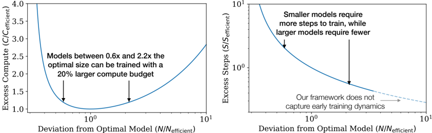
## Chart/Diagram Type: Dual-Plot Analysis of Model Efficiency ### Overview The image contains two side-by-side graphs analyzing model efficiency. The left plot examines **excess compute** relative to deviation from an optimal model size, while the right plot analyzes **excess training steps** under the same deviation metric. Both graphs use logarithmic scales on the x-axis and linear/logarithmic scales on the y-axis, with annotations highlighting key insights. --- ### Components/Axes #### Left Plot (Excess Compute) - **Y-axis**: "Excess Compute (C/C_efficient)" (linear scale, 1.0–4.0) - **X-axis**: "Deviation from Optimal Model (N/N_efficient)" (logarithmic scale, 10⁰–10¹) - **Legend**: No explicit legend; single blue line represents the efficiency curve. - **Annotations**: - Text: "Models between 0.6x and 2.2x the optimal size can be trained with a 20% larger compute budget." - Two arrows point to the minimum of the curve (at ~1.0 on the x-axis). #### Right Plot (Excess Steps) - **Y-axis**: "Excess Steps (S/S_efficient)" (logarithmic scale, 10⁰–10¹) - **X-axis**: "Deviation from Optimal Model (N/N_efficient)" (logarithmic scale, 10⁰–10¹) - **Legend**: No explicit legend; single blue line represents the efficiency curve. - **Annotations**: - Text: "Smaller models require more steps to train, while larger models require fewer." - Arrow points to a specific deviation value (~1.5 on the x-axis). - Dashed line with text: "Our framework does not capture early training dynamics." --- ### Detailed Analysis #### Left Plot Trends - The curve starts at ~4.0 excess compute when deviation is 10⁰ (optimal model size). - Excess compute sharply decreases as deviation increases, reaching a minimum of ~1.0 at ~1.0 deviation. - Beyond ~1.0 deviation, excess compute rises again, plateauing near ~2.5 at 10¹ deviation. - The annotation indicates that models within 0.6x–2.2x the optimal size require only a 20% larger compute budget, suggesting a "sweet spot" for efficiency. #### Right Plot Trends - The curve starts at ~10¹ excess steps at 10⁰ deviation (optimal model size). - Excess steps decrease logarithmically as deviation increases, dropping to ~10⁰ at ~1.5 deviation. - Beyond ~1.5 deviation, the curve flattens, indicating diminishing returns in step efficiency. - The annotation highlights that smaller models (deviation <1.0) require exponentially more steps, while larger models (deviation >1.0) require fewer steps. --- ### Key Observations 1. **Optimal Model Size**: Both plots converge at ~1.0 deviation, where compute and step efficiency are minimized. 2. **Compute vs. Steps Tradeoff**: - Smaller models (deviation <1.0) require disproportionately more compute and steps. - Larger models (deviation >1.0) show improved efficiency but face diminishing returns. 3. **Framework Limitation**: The dashed line in the right plot explicitly states that early training dynamics (e.g., initial learning phases) are not modeled. --- ### Interpretation The data suggests that **model size optimization is critical for balancing compute and training efficiency**. The "sweet spot" (0.6x–2.2x optimal size) minimizes excess compute, but training steps remain highly sensitive to deviations below the optimal size. The framework’s inability to model early training dynamics implies potential gaps in understanding how model size impacts initial learning phases, which could affect real-world deployment strategies. The logarithmic x-axis emphasizes that even small deviations from the optimal size have nonlinear impacts, particularly for smaller models. This aligns with the observation that smaller models require exponentially more resources, reinforcing the importance of targeting near-optimal sizes in practice.