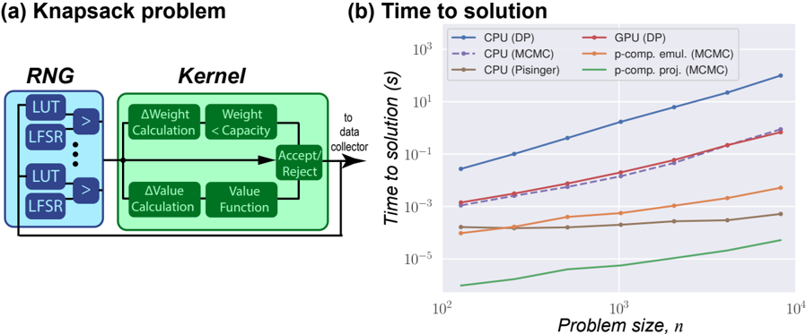
## Diagram and Chart: Knapsack Problem and Time to Solution ### Overview The image presents two sub-figures: (a) a diagram illustrating the components of a Knapsack problem solver, and (b) a chart comparing the time to solution for different algorithms (CPU and GPU implementations) as a function of problem size. ### Components/Axes #### (a) Knapsack Problem Diagram * **Title:** Knapsack problem * **Components:** * **RNG (Random Number Generator):** Contains multiple LUT (Look-Up Table) and LFSR (Linear Feedback Shift Register) pairs. Arrows indicate data flow from each LUT/LFSR pair to a comparator (>). * **Kernel:** Contains two parallel processes: * **Top Branch:** ΔWeight Calculation followed by Weight < Capacity comparison. * **Bottom Branch:** ΔValue Calculation followed by Value Function. * **Accept/Reject:** A decision block that receives input from both branches of the Kernel. * **Data Flow:** The output of the Accept/Reject block is fed back into the Kernel, creating a loop. The output also goes "to data collector". #### (b) Time to Solution Chart * **Title:** Time to solution * **X-axis:** Problem size, *n*. Logarithmic scale from approximately 10² to 10⁴. Axis markers at 10², 10³, and 10⁴. * **Y-axis:** Time to solution (s). Logarithmic scale from approximately 10^-5 to 10³. Axis markers at 10^-5, 10^-3, 10^-1, 10¹, and 10³. * **Legend (Top-Left):** * Blue solid line: CPU (DP) * Purple dashed line: CPU (MCMC) * Brown solid line: CPU (Pisinger) * Red solid line: GPU (DP) * Orange solid line: p-comp. emul. (MCMC) * Green solid line: p-comp. proj. (MCMC) ### Detailed Analysis #### (a) Knapsack Problem Diagram The diagram illustrates the core components of a knapsack problem solver. The RNG generates random numbers used by the Kernel to evaluate potential solutions. The Kernel calculates changes in weight and value, and the Accept/Reject block determines whether to accept the new solution or reject it. The feedback loop allows the algorithm to iteratively refine the solution. #### (b) Time to Solution Chart * **CPU (DP) - Blue Solid Line:** The time to solution increases rapidly with problem size. * At n = 100, time ≈ 0.03 s * At n = 1000, time ≈ 1 s * At n = 10000, time ≈ 100 s * **CPU (MCMC) - Purple Dashed Line:** The time to solution increases rapidly with problem size, but is lower than CPU (DP). * At n = 100, time ≈ 0.001 s * At n = 1000, time ≈ 0.03 s * At n = 10000, time ≈ 3 s * **CPU (Pisinger) - Brown Solid Line:** The time to solution remains relatively constant with problem size. * At n = 100, time ≈ 0.00003 s * At n = 1000, time ≈ 0.00005 s * At n = 10000, time ≈ 0.0001 s * **GPU (DP) - Red Solid Line:** The time to solution increases rapidly with problem size, and is lower than CPU (DP). * At n = 100, time ≈ 0.001 s * At n = 1000, time ≈ 0.03 s * At n = 10000, time ≈ 3 s * **p-comp. emul. (MCMC) - Orange Solid Line:** The time to solution remains relatively constant with problem size. * At n = 100, time ≈ 0.00005 s * At n = 1000, time ≈ 0.0002 s * At n = 10000, time ≈ 0.001 s * **p-comp. proj. (MCMC) - Green Solid Line:** The time to solution remains relatively constant with problem size. * At n = 100, time ≈ 0.00001 s * At n = 1000, time ≈ 0.00002 s * At n = 10000, time ≈ 0.00005 s ### Key Observations * The CPU (DP) algorithm has the highest time to solution, increasing dramatically with problem size. * The CPU (MCMC) and GPU (DP) algorithms have similar performance, with the GPU implementation being slightly faster. * The CPU (Pisinger), p-comp. emul. (MCMC), and p-comp. proj. (MCMC) algorithms have significantly lower time to solution, and their performance is relatively independent of problem size. ### Interpretation The chart demonstrates the performance differences between various algorithms for solving the Knapsack problem. Dynamic Programming (DP) implementations (CPU and GPU) exhibit a steep increase in time to solution as the problem size grows, indicating a higher computational complexity. Markov Chain Monte Carlo (MCMC) methods, especially when parallelized (p-comp. emul. and p-comp. proj.), show a much flatter curve, suggesting better scalability for larger problem instances. The Pisinger algorithm on the CPU also shows excellent performance and scalability. The data suggests that for larger Knapsack problems, MCMC-based or Pisinger algorithms are significantly more efficient than DP-based approaches. The GPU implementation of DP offers a modest improvement over the CPU version, but the algorithmic choice has a much greater impact on performance.

## Diagram & Chart: Knapsack Problem & Time to Solution ### Overview The image presents a diagram illustrating the components of a Knapsack problem solver, alongside a chart showing the time to solution for different algorithms as a function of problem size. The diagram details the Random Number Generator (RNG) and Kernel components, while the chart compares the performance of CPU and GPU implementations using different methods. ### Components/Axes **Diagram:** * **Header:** "Knapsack problem" * **Left Block:** "RNG" containing "LUT" and "LFSR" repeated multiple times. Arrows indicate flow. * **Right Block:** "Kernel" containing "ΔWeight Calculation", "Weight < Capacity", "Accept/Reject", "ΔValue Calculation", "Value Function". Arrows indicate flow. * **Connections:** Arrows connect the RNG to the Kernel for both weight and value calculations. An arrow leads from "Accept/Reject" to "to data collector". **Chart:** * **Title:** "Time to solution" * **X-axis:** "Problem size, n" (logarithmic scale, ranging from 10² to 10⁴) * **Y-axis:** "Time to solution (s)" (logarithmic scale, ranging from 10^-5 to 10¹) * **Legend (top-right):** * Blue Solid Line: "CPU (DP)" * Red Solid Line: "GPU (DP)" * Orange Dashed Line: "CPU (MCMC)" * Yellow Dashed Line: "p-comp. emul. (MCMC)" * Green Solid Line: "CPU (Pisinger)" * Teal Dashed Line: "p-comp. proj. (MCMC)" ### Detailed Analysis or Content Details **Diagram:** The diagram illustrates a system for solving the Knapsack problem. The "RNG" block generates random numbers using Look-Up Tables (LUTs) and Linear Feedback Shift Registers (LFSRs). These random numbers are fed into the "Kernel" block, where weight and value differences are calculated. The calculated weight is compared against the "Capacity". Based on this comparison, solutions are either "Accept"ed or "Reject"ed and sent to a "data collector". **Chart:** * **CPU (DP) (Blue Solid Line):** Starts at approximately 0.1 seconds at n=10², increases steadily to approximately 10 seconds at n=10⁴. The line is nearly linear on this log-log scale. * **GPU (DP) (Red Solid Line):** Starts at approximately 0.01 seconds at n=10², increases to approximately 0.1 seconds at n=10⁴. The line is nearly linear on this log-log scale. * **CPU (MCMC) (Orange Dashed Line):** Starts at approximately 0.001 seconds at n=10², increases to approximately 0.01 seconds at n=10⁴. The line is relatively flat. * **p-comp. emul. (MCMC) (Yellow Dashed Line):** Starts at approximately 0.0005 seconds at n=10², increases to approximately 0.005 seconds at n=10⁴. The line is relatively flat. * **CPU (Pisinger) (Green Solid Line):** Starts at approximately 0.00001 seconds at n=10², increases to approximately 0.0001 seconds at n=10⁴. The line is nearly flat. * **p-comp. proj. (MCMC) (Teal Dashed Line):** Starts at approximately 0.000005 seconds at n=10², increases to approximately 0.00005 seconds at n=10⁴. The line is nearly flat. ### Key Observations * The CPU (DP) method is significantly slower than all other methods, especially as the problem size increases. * The GPU (DP) method is faster than the CPU (DP) method, but still slower than the MCMC-based methods. * The MCMC-based methods (CPU (MCMC), p-comp. emul. (MCMC), CPU (Pisinger), and p-comp. proj. (MCMC)) exhibit relatively constant solution times regardless of problem size. * The "p-comp. proj. (MCMC)" method is the fastest across all problem sizes. * The chart uses a logarithmic scale for both axes, indicating a wide range of values. ### Interpretation The data suggests that for solving the Knapsack problem, Dynamic Programming (DP) is computationally expensive and scales poorly with problem size. The GPU implementation of DP offers some improvement over the CPU implementation, but the performance is still limited. Markov Chain Monte Carlo (MCMC) methods, particularly the "p-comp. proj. (MCMC)" variant, provide a much more efficient solution, with solution times remaining relatively constant even as the problem size increases. This indicates that MCMC methods are better suited for large-scale Knapsack problems. The diagram illustrates the underlying process of the Knapsack solver, highlighting the role of random number generation and the iterative acceptance/rejection process within the Kernel. The connection between the RNG and the Kernel suggests that the quality of the random numbers is crucial for the performance of the solver. The "Accept/Reject" step implies a probabilistic approach to finding optimal solutions, which is consistent with the use of MCMC methods. The "to data collector" arrow indicates that the accepted solutions are accumulated for analysis.

## [Chart/Diagram Type]: Technical Diagram and Performance Chart ### Overview The image is a composite figure containing two distinct parts. Part (a) is a block diagram illustrating the computational flow of a "Knapsack problem" solver. Part (b) is a line chart titled "Time to solution," comparing the performance of different computational methods (CPU and GPU-based) for solving the knapsack problem as the problem size increases. ### Components/Axes #### Part (a): Knapsack problem Diagram * **Title:** "(a) Knapsack problem" * **Main Blocks:** * **RNG (Random Number Generator):** A blue box on the left containing multiple stacked sub-blocks. Each sub-block contains a "LUT" (Look-Up Table) and an "LFSR" (Linear Feedback Shift Register), connected by an arrow. An ellipsis (`...`) indicates multiple such units. * **Kernel:** A green box on the right. It contains four internal calculation blocks: * `ΔWeight Calculation` * `Weight < Capacity` * `ΔValue Calculation` * `Value Function` * **Decision Block:** A smaller green box labeled `Accept/Reject`, which receives input from the `Weight < Capacity` and `Value Function` blocks. * **Data Flow:** 1. Arrows flow from the RNG block into the Kernel. 2. Inside the Kernel, parallel paths lead to the `Accept/Reject` decision. 3. An arrow exits the `Accept/Reject` block, labeled "to data collector". 4. A feedback loop arrow returns from the "to data collector" line back to the input of the Kernel. #### Part (b): Time to solution Chart * **Title:** "(b) Time to solution" * **X-Axis:** * **Label:** `Problem size, n` * **Scale:** Logarithmic, ranging from `10^2` to `10^4`. * **Major Ticks:** `10^2`, `10^3`, `10^4`. * **Y-Axis:** * **Label:** `Time to solution (s)` * **Scale:** Logarithmic, ranging from `10^-5` to `10^3` seconds. * **Major Ticks:** `10^-5`, `10^-3`, `10^-1`, `10^1`, `10^3`. * **Legend (Top-Left Corner):** Contains six entries, each with a distinct color and line/marker style. 1. `CPU (DP)` - Blue line with circular markers. 2. `CPU (MCMC)` - Purple dashed line with circular markers. 3. `CPU (Pisinger)` - Brown line with circular markers. 4. `GPU (DP)` - Red line with circular markers. 5. `p-comp. emul. (MCMC)` - Orange line with circular markers. 6. `p-comp. proj. (MCMC)` - Green line with circular markers. ### Detailed Analysis #### Part (a): Diagram Content The diagram depicts a stochastic optimization algorithm for the knapsack problem. The **RNG** block generates random numbers using LUTs and LFSRs, which are fed into the **Kernel**. The Kernel performs core calculations: it computes the change in weight (`ΔWeight`) and value (`ΔValue`) for a potential item, checks if the new weight is within capacity (`Weight < Capacity`), and evaluates the item's value (`Value Function`). Based on these checks, the `Accept/Reject` block decides whether to include the item. The result is sent to a data collector, and the process loops. #### Part (b): Chart Data & Trends * **General Trend:** All six data series show an increase in "Time to solution" as "Problem size, n" increases. The relationship appears linear on this log-log plot, suggesting a power-law relationship (Time ∝ n^k). * **Series Performance (from slowest to fastest at n=10^4):** 1. **CPU (DP) [Blue]:** The slowest method. At n=10^2, time is ~10^-1.5 s (~0.03 s). At n=10^4, time is ~10^2.5 s (~316 s). It has the steepest slope. 2. **GPU (DP) [Red] & CPU (MCMC) [Purple Dashed]:** These two lines are very close, with GPU (DP) slightly faster. At n=10^2, both are ~10^-3 s. At n=10^4, both are ~10^0 s (1 s). Their slopes are similar and less steep than CPU (DP). 3. **p-comp. emul. (MCMC) [Orange]:** Significantly faster. At n=10^2, time is ~10^-4 s. At n=10^4, time is ~10^-2.5 s (~0.003 s). 4. **CPU (Pisinger) [Brown]:** Faster still. At n=10^2, time is ~10^-4 s. At n=10^4, time is ~10^-3.5 s (~0.0003 s). Its slope is very shallow. 5. **p-comp. proj. (MCMC) [Green]:** The fastest method by a large margin. At n=10^2, time is ~10^-5.5 s (~3e-6 s). At n=10^4, time is ~10^-4.5 s (~3e-5 s). It has the shallowest slope. ### Key Observations 1. **Massive Performance Gap:** There is a performance difference of over 7 orders of magnitude (~10 million times) between the slowest (CPU DP) and fastest (p-comp. proj. MCMC) methods at n=10^4. 2. **Algorithm Efficiency:** The "p-comp. proj. (MCMC)" method (likely a quantum-inspired or probabilistic computing projection) demonstrates exceptional scalability, with time increasing very slowly with problem size. 3. **Hardware vs. Algorithm:** While the GPU accelerates the Dynamic Programming (DP) algorithm compared to the CPU, the algorithmic choice (MCMC vs. DP) and computing paradigm (p-comp. vs. classical) have a far greater impact on performance than the hardware (CPU vs. GPU) alone. 4. **Specialized Solver:** The "CPU (Pisinger)" line likely represents a highly optimized, specialized classical algorithm for the knapsack problem, outperforming generic MCMC on a CPU. ### Interpretation This figure makes a compelling case for the use of advanced, possibly quantum-inspired, probabilistic computing methods (`p-comp. proj. (MCMC)`) for solving combinatorial optimization problems like the knapsack problem. The data suggests that as problem size scales, traditional exact methods (DP) become computationally intractable, while specialized classical heuristics (Pisinger) offer good performance. However, the projected probabilistic computing approach offers a paradigm shift, providing solutions in near-constant time relative to the problem size within the tested range. The diagram in (a) likely represents the internal workflow of one of these MCMC-based solvers, showing how random sampling (RNG) is used within an iterative kernel to explore the solution space and make accept/reject decisions. The combination of (a) and (b) argues that the architecture shown in (a), when implemented on a suitable probabilistic computing platform, yields the dramatic performance gains illustrated in (b).

## Diagram and Chart Analysis: Knapsack Problem and Computational Efficiency ### Overview The image contains two components: 1. **Diagram (a)**: A flowchart titled "Knapsack problem" illustrating algorithmic steps. 2. **Chart (b)**: A line graph titled "Time to solution" comparing computational methods across problem sizes. --- ### Components/Axes #### Diagram (a) - **Blocks**: - **RNG**: Contains "LUT" and "LFSR" (repeated). - **Kernel**: Contains: - ΔWeight Calculation → Weight < Capacity - ΔValue Calculation → Value Function - Accept/Reject decision node. - **Flow**: - RNG → LUT/LFSR → Kernel (calculations) → Accept/Reject → Data collector. #### Chart (b) - **X-axis**: Problem size, *n* (log scale: 10² to 10⁴). - **Y-axis**: Time to solution (log scale: 10⁻⁵ to 10³ seconds). - **Legend**: - **Blue**: CPU (DP) - **Red**: GPU (DP) - **Purple (dashed)**: CPU (MCMC) - **Orange**: p-comp. emul. (MCMC) - **Brown**: CPU (Pisinger) - **Green**: p-comp. proj. (MCMC) --- ### Detailed Analysis #### Diagram (a) - **Textual Elements**: - "ΔWeight Calculation", "Weight < Capacity", "ΔValue Calculation", "Value Function", "Accept/Reject". - Arrows indicate sequential flow from RNG to Kernel to data collector. #### Chart (b) - **Data Series Trends**: 1. **CPU (DP) (Blue)**: Steep upward slope. At *n=10²*, ~10⁻³ s; at *n=10⁴*, ~10³ s. 2. **GPU (DP) (Red)**: Moderate upward slope. At *n=10²*, ~10⁻³ s; at *n=10⁴*, ~10¹ s. 3. **CPU (MCMC) (Purple, dashed)**: Slight upward curve. At *n=10²*, ~10⁻⁴ s; at *n=10⁴*, ~10⁰ s. 4. **p-comp. emul. (MCMC) (Orange)**: Flat then slight rise. At *n=10²*, ~10⁻⁵ s; at *n=10⁴*, ~10⁻² s. 5. **CPU (Pisinger) (Brown)**: Flat line. ~10⁻⁵ s across all *n*. 6. **p-comp. proj. (MCMC) (Green)**: Gradual upward curve. At *n=10²*, ~10⁻⁶ s; at *n=10⁴*, ~10⁻³ s. --- ### Key Observations 1. **CPU (DP)** exhibits exponential growth in time with problem size. 2. **p-comp. proj. (MCMC)** (green line) is the most efficient, scaling sub-linearly. 3. **CPU (Pisinger)** (brown line) remains constant, suggesting fixed computational cost. 4. **GPU (DP)** (red line) outperforms CPU (DP) but lags behind MCMC methods. --- ### Interpretation - **Diagram (a)**: The knapsack problem workflow involves random number generation (RNG), look-up tables (LUT), and lightweight feedback shift registers (LFSR) to drive kernel computations. The kernel evaluates weight/value constraints and decides whether to accept/reject solutions, feeding results to a data collector. - **Chart (b)**: Computational efficiency varies significantly by method. CPU (DP) becomes impractical for large *n* (e.g., 10⁴), while p-comp. proj. (MCMC) scales efficiently. The constant time for CPU (Pisinger) suggests a specialized optimization. - **Notable Anomaly**: The dashed purple line (CPU MCMC) initially outperforms GPU (DP) but diverges at larger *n*. This analysis highlights trade-offs between algorithmic design (diagram) and computational scalability (chart), emphasizing the importance of method selection for problem size.