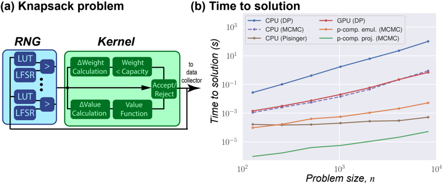
## Diagram and Chart: Knapsack Problem and Time to Solution ### Overview The image presents two sub-figures: (a) a diagram illustrating the components of a Knapsack problem solver, and (b) a chart comparing the time to solution for different algorithms (CPU and GPU implementations) as a function of problem size. ### Components/Axes #### (a) Knapsack Problem Diagram * **Title:** Knapsack problem * **Components:** * **RNG (Random Number Generator):** Contains multiple LUT (Look-Up Table) and LFSR (Linear Feedback Shift Register) pairs. Arrows indicate data flow from each LUT/LFSR pair to a comparator (>). * **Kernel:** Contains two parallel processes: * **Top Branch:** ΔWeight Calculation followed by Weight < Capacity comparison. * **Bottom Branch:** ΔValue Calculation followed by Value Function. * **Accept/Reject:** A decision block that receives input from both branches of the Kernel. * **Data Flow:** The output of the Accept/Reject block is fed back into the Kernel, creating a loop. The output also goes "to data collector". #### (b) Time to Solution Chart * **Title:** Time to solution * **X-axis:** Problem size, *n*. Logarithmic scale from approximately 10² to 10⁴. Axis markers at 10², 10³, and 10⁴. * **Y-axis:** Time to solution (s). Logarithmic scale from approximately 10^-5 to 10³. Axis markers at 10^-5, 10^-3, 10^-1, 10¹, and 10³. * **Legend (Top-Left):** * Blue solid line: CPU (DP) * Purple dashed line: CPU (MCMC) * Brown solid line: CPU (Pisinger) * Red solid line: GPU (DP) * Orange solid line: p-comp. emul. (MCMC) * Green solid line: p-comp. proj. (MCMC) ### Detailed Analysis #### (a) Knapsack Problem Diagram The diagram illustrates the core components of a knapsack problem solver. The RNG generates random numbers used by the Kernel to evaluate potential solutions. The Kernel calculates changes in weight and value, and the Accept/Reject block determines whether to accept the new solution or reject it. The feedback loop allows the algorithm to iteratively refine the solution. #### (b) Time to Solution Chart * **CPU (DP) - Blue Solid Line:** The time to solution increases rapidly with problem size. * At n = 100, time ≈ 0.03 s * At n = 1000, time ≈ 1 s * At n = 10000, time ≈ 100 s * **CPU (MCMC) - Purple Dashed Line:** The time to solution increases rapidly with problem size, but is lower than CPU (DP). * At n = 100, time ≈ 0.001 s * At n = 1000, time ≈ 0.03 s * At n = 10000, time ≈ 3 s * **CPU (Pisinger) - Brown Solid Line:** The time to solution remains relatively constant with problem size. * At n = 100, time ≈ 0.00003 s * At n = 1000, time ≈ 0.00005 s * At n = 10000, time ≈ 0.0001 s * **GPU (DP) - Red Solid Line:** The time to solution increases rapidly with problem size, and is lower than CPU (DP). * At n = 100, time ≈ 0.001 s * At n = 1000, time ≈ 0.03 s * At n = 10000, time ≈ 3 s * **p-comp. emul. (MCMC) - Orange Solid Line:** The time to solution remains relatively constant with problem size. * At n = 100, time ≈ 0.00005 s * At n = 1000, time ≈ 0.0002 s * At n = 10000, time ≈ 0.001 s * **p-comp. proj. (MCMC) - Green Solid Line:** The time to solution remains relatively constant with problem size. * At n = 100, time ≈ 0.00001 s * At n = 1000, time ≈ 0.00002 s * At n = 10000, time ≈ 0.00005 s ### Key Observations * The CPU (DP) algorithm has the highest time to solution, increasing dramatically with problem size. * The CPU (MCMC) and GPU (DP) algorithms have similar performance, with the GPU implementation being slightly faster. * The CPU (Pisinger), p-comp. emul. (MCMC), and p-comp. proj. (MCMC) algorithms have significantly lower time to solution, and their performance is relatively independent of problem size. ### Interpretation The chart demonstrates the performance differences between various algorithms for solving the Knapsack problem. Dynamic Programming (DP) implementations (CPU and GPU) exhibit a steep increase in time to solution as the problem size grows, indicating a higher computational complexity. Markov Chain Monte Carlo (MCMC) methods, especially when parallelized (p-comp. emul. and p-comp. proj.), show a much flatter curve, suggesting better scalability for larger problem instances. The Pisinger algorithm on the CPU also shows excellent performance and scalability. The data suggests that for larger Knapsack problems, MCMC-based or Pisinger algorithms are significantly more efficient than DP-based approaches. The GPU implementation of DP offers a modest improvement over the CPU version, but the algorithmic choice has a much greater impact on performance.