## Diagram and Chart Analysis: Knapsack Problem and Computational Efficiency
### Overview
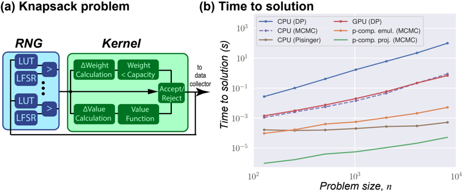
The image contains two components:
1. **Diagram (a)**: A flowchart titled "Knapsack problem" illustrating algorithmic steps.
2. **Chart (b)**: A line graph titled "Time to solution" comparing computational methods across problem sizes.
---
### Components/Axes
#### Diagram (a)
- **Blocks**:
- **RNG**: Contains "LUT" and "LFSR" (repeated).
- **Kernel**: Contains:
- ΔWeight Calculation → Weight < Capacity
- ΔValue Calculation → Value Function
- Accept/Reject decision node.
- **Flow**:
- RNG → LUT/LFSR → Kernel (calculations) → Accept/Reject → Data collector.
#### Chart (b)
- **X-axis**: Problem size, *n* (log scale: 10² to 10⁴).
- **Y-axis**: Time to solution (log scale: 10⁻⁵ to 10³ seconds).
- **Legend**:
- **Blue**: CPU (DP)
- **Red**: GPU (DP)
- **Purple (dashed)**: CPU (MCMC)
- **Orange**: p-comp. emul. (MCMC)
- **Brown**: CPU (Pisinger)
- **Green**: p-comp. proj. (MCMC)
---
### Detailed Analysis
#### Diagram (a)
- **Textual Elements**:
- "ΔWeight Calculation", "Weight < Capacity", "ΔValue Calculation", "Value Function", "Accept/Reject".
- Arrows indicate sequential flow from RNG to Kernel to data collector.
#### Chart (b)
- **Data Series Trends**:
1. **CPU (DP) (Blue)**: Steep upward slope. At *n=10²*, ~10⁻³ s; at *n=10⁴*, ~10³ s.
2. **GPU (DP) (Red)**: Moderate upward slope. At *n=10²*, ~10⁻³ s; at *n=10⁴*, ~10¹ s.
3. **CPU (MCMC) (Purple, dashed)**: Slight upward curve. At *n=10²*, ~10⁻⁴ s; at *n=10⁴*, ~10⁰ s.
4. **p-comp. emul. (MCMC) (Orange)**: Flat then slight rise. At *n=10²*, ~10⁻⁵ s; at *n=10⁴*, ~10⁻² s.
5. **CPU (Pisinger) (Brown)**: Flat line. ~10⁻⁵ s across all *n*.
6. **p-comp. proj. (MCMC) (Green)**: Gradual upward curve. At *n=10²*, ~10⁻⁶ s; at *n=10⁴*, ~10⁻³ s.
---
### Key Observations
1. **CPU (DP)** exhibits exponential growth in time with problem size.
2. **p-comp. proj. (MCMC)** (green line) is the most efficient, scaling sub-linearly.
3. **CPU (Pisinger)** (brown line) remains constant, suggesting fixed computational cost.
4. **GPU (DP)** (red line) outperforms CPU (DP) but lags behind MCMC methods.
---
### Interpretation
- **Diagram (a)**: The knapsack problem workflow involves random number generation (RNG), look-up tables (LUT), and lightweight feedback shift registers (LFSR) to drive kernel computations. The kernel evaluates weight/value constraints and decides whether to accept/reject solutions, feeding results to a data collector.
- **Chart (b)**: Computational efficiency varies significantly by method. CPU (DP) becomes impractical for large *n* (e.g., 10⁴), while p-comp. proj. (MCMC) scales efficiently. The constant time for CPU (Pisinger) suggests a specialized optimization.
- **Notable Anomaly**: The dashed purple line (CPU MCMC) initially outperforms GPU (DP) but diverges at larger *n*.
This analysis highlights trade-offs between algorithmic design (diagram) and computational scalability (chart), emphasizing the importance of method selection for problem size.