## Diagram: Transformer Layer Architecture with MLP and Redistribution Effect
### Overview
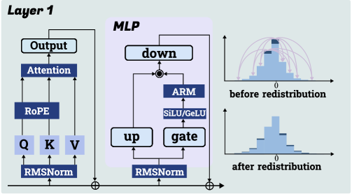
This image is a technical diagram illustrating the architecture of a single transformer layer (labeled "Layer 1") with a specific Multi-Layer Perceptron (MLP) block, alongside two histograms demonstrating a data redistribution effect. The diagram is divided into three primary regions: the main transformer layer flow on the left, the detailed MLP block in the center, and two comparative histograms on the right.
### Components/Axes
**Left Region: Layer 1**
* **Title:** "Layer 1" (top-left corner).
* **Components (from bottom to top):**
* `RMSNorm` (Root Mean Square Normalization) block at the base.
* Three parallel paths leading to `Q`, `K`, `V` (Query, Key, Value) blocks.
* `RoPE` (Rotary Positional Embedding) block above Q, K, V.
* `Attention` block above RoPE.
* `Output` block at the top.
* **Flow:** Data flows upward from `RMSNorm` through `Q/K/V` -> `RoPE` -> `Attention` -> `Output`. A residual connection (indicated by a circled plus `⊕`) bypasses the entire attention block, adding the original input to the `Output`.
**Center Region: MLP Block**
* **Title:** "MLP" (top-left of the shaded box).
* **Components:**
* `RMSNorm` block at the base.
* Two parallel paths from `RMSNorm`: one to an `up` projection block and one to a `gate` block.
* `SiLU/GELU` activation function block above `gate`.
* `ARM` block (likely an Adaptive or Attention-based Redistribution Module) above the activation.
* `down` projection block at the top.
* **Flow:** The outputs of the `up` path and the `gate` -> `SiLU/GELU` -> `ARM` path are combined via element-wise multiplication (indicated by `⊗`). This combined signal then goes to the `down` block. A residual connection (`⊕`) bypasses the entire MLP block, adding the original input to the `down` output.
**Right Region: Histograms**
* **Top Histogram:**
* **Title/Label:** "before redistribution" (below the plot).
* **X-axis:** Centered at `0`.
* **Visual:** A blue histogram showing a distribution of values. Several red, curved arrows originate from the tails of the distribution and point towards the center, suggesting a process that pulls extreme values inward.
* **Bottom Histogram:**
* **Title/Label:** "after redistribution" (below the plot).
* **X-axis:** Centered at `0`.
* **Visual:** A blue histogram showing a distribution that is more concentrated (narrower) around the central `0` value compared to the "before" histogram.
### Detailed Analysis
**Architectural Flow:**
1. The main "Layer 1" processes input through a standard transformer sub-layer: `RMSNorm` -> `Q/K/V` projections -> `RoPE` -> `Attention` -> `Output`, with a residual connection.
2. The output of the attention sub-layer is then fed into the specialized "MLP" block.
3. Within the MLP, the input is normalized again (`RMSNorm`). It is then processed by two parallel paths: a standard `up` projection and a gated path (`gate` -> `SiLU/GELU` -> `ARM`). The `ARM` module is a key component, positioned after the activation function.
4. The outputs of these two paths are multiplied (`⊗`) and then projected back down via the `down` block. A final residual connection adds the MLP's input to its output.
**Redistribution Effect:**
The histograms visually demonstrate the function of the `ARM` module within the MLP.
* **Before Redistribution:** The data distribution has wider tails, with values spread further from zero. The red arrows symbolize the `ARM`'s intended action: redistributing mass from the tails towards the center.
* **After Redistribution:** The resulting distribution is tighter and more peaked around zero, confirming the effect of the `ARM` in concentrating the data values.
### Key Observations
1. **Component Integration:** The `ARM` is not a standalone block but is integrated into the gated linear unit (GLU) pathway of the MLP, specifically after the non-linear activation (`SiLU/GELU`).
2. **Dual Normalization:** The architecture employs `RMSNorm` twice: once at the very beginning of the layer (before attention) and again at the beginning of the MLP block.
3. **Residual Connections:** Standard residual connections (`⊕`) are present for both the attention and MLP sub-layers, which is typical for transformer architectures.
4. **Visual Metaphor:** The red arrows in the "before" histogram are a clear visual metaphor for a "pulling" or "constraining" force acting on outlier values.
### Interpretation
This diagram describes a modified transformer layer designed to control the distribution of activations within the MLP block. The core innovation appears to be the **ARM (Adaptive Redistribution Module)**.
* **Purpose:** The primary goal is to mitigate the issue of activation outliers or excessive spread in the value distribution, which can hinder model training stability and efficiency. By redistributing mass from the tails to the center, the ARM likely promotes more stable gradients and potentially allows for lower-precision computation.
* **Mechanism:** The ARM operates within the gating mechanism of a SwiGLU/GELU-style MLP. It acts on the activated values before they are modulated by the up-projection and before the final down-projection. This placement suggests it directly shapes the information flow through the MLP.
* **Relationship:** The left and center diagrams show the *structural* implementation (where the ARM is placed), while the right histograms show the *functional* outcome (what the ARM does to the data). The connection is causal: the architecture on the left produces the effect shown on the right.
* **Significance:** This technique is relevant for improving large language model (LLM) training and inference. Controlling activation distributions can lead to more robust models, easier quantization, and reduced computational overhead. The diagram succinctly communicates both the "how" (architecture) and the "why" (distributional effect) of this modification.