## Line Chart: k-shot Regression Performance (k=10)
### Overview
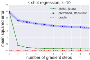
The image is a line chart comparing the performance of three different methods for a k-shot regression task with k=10. The chart plots the mean squared error (MSE) against the number of gradient steps taken during adaptation. The primary comparison is between a proposed method ("MAML (ours)") and a "pretrained" baseline, with an "oracle" representing the theoretical best performance.
### Components/Axes
* **Chart Title:** "k-shot regression, k=10" (centered at the top).
* **Y-Axis:**
* **Label:** "mean squared error" (rotated vertically on the left).
* **Scale:** Linear scale from 0 to 35, with major tick marks at intervals of 5 (0, 5, 10, 15, 20, 25, 30, 35).
* **X-Axis:**
* **Label:** "number of gradient steps" (centered at the bottom).
* **Scale:** Linear scale from 0 to 9, with integer tick marks for each step (0, 1, 2, ..., 9).
* **Legend:** Located in the top-right corner of the plot area. It contains three entries:
1. **Green solid line with circular markers:** "MAML (ours)"
2. **Blue dashed line with square markers:** "pretrained, step=0.02"
3. **Red dotted line with diamond markers:** "oracle"
* **Grid:** A light gray grid is present in the background.
### Detailed Analysis
The chart displays three distinct data series, each showing a different trend in mean squared error as the number of gradient steps increases.
1. **MAML (ours) - Green Solid Line:**
* **Trend:** Shows a very rapid, steep decline in error initially, followed by a plateau near zero.
* **Data Points (Approximate):**
* Step 0: MSE ≈ 30
* Step 1: MSE ≈ 2 (dramatic drop)
* Step 2: MSE ≈ 1
* Step 3: MSE ≈ 0.8
* Step 4: MSE ≈ 0.6
* Step 5: MSE ≈ 0.5
* Step 6: MSE ≈ 0.4
* Step 7: MSE ≈ 0.3
* Step 8: MSE ≈ 0.2
* Step 9: MSE ≈ 0.1
2. **pretrained, step=0.02 - Blue Dashed Line:**
* **Trend:** Shows a steady, gradual decline in error, but remains significantly higher than the MAML method throughout.
* **Data Points (Approximate):**
* Step 0: MSE ≈ 30
* Step 1: MSE ≈ 23
* Step 2: MSE ≈ 21
* Step 3: MSE ≈ 20
* Step 4: MSE ≈ 19.5
* Step 5: MSE ≈ 19
* Step 6: MSE ≈ 18.5
* Step 7: MSE ≈ 18
* Step 8: MSE ≈ 17.5
* Step 9: MSE ≈ 17
3. **oracle - Red Dotted Line:**
* **Trend:** A flat, horizontal line at the very bottom of the chart, representing constant, near-zero error.
* **Data Points:** Consistently at MSE ≈ 0 for all gradient steps (0 through 9).
### Key Observations
* **Convergence Speed:** The "MAML (ours)" method converges extremely quickly, achieving near-oracle performance within just 1-2 gradient steps.
* **Performance Gap:** A large and persistent performance gap exists between the "pretrained" baseline and the "MAML" method. After 9 steps, the pretrained model's error (~17) is still orders of magnitude higher than MAML's error (~0.1).
* **Starting Point:** All three methods appear to start from a similar high-error state (MSE ≈ 30) at step 0, before any task-specific gradient steps are applied.
* **Oracle Baseline:** The "oracle" line provides a clear lower bound, showing the best possible performance achievable.
### Interpretation
This chart demonstrates the superior few-shot learning capability of the MAML (Model-Agnostic Meta-Learning) algorithm compared to a standard pretrained model in a regression setting.
* **What the data suggests:** The data strongly suggests that MAML is highly efficient at adapting to new tasks with very limited data (10 examples, as k=10). Its internal meta-learned initialization allows it to reach optimal performance with minimal computation (1-2 steps). In contrast, the pretrained model, while improving, adapts slowly and inefficiently, indicating its learned representations are not as readily adaptable for this specific task.
* **How elements relate:** The x-axis (gradient steps) represents the adaptation effort. The y-axis (MSE) represents the cost of errors. The steep green curve shows that MAML converts adaptation effort into performance gain very effectively. The shallow blue curve shows the pretrained model requires much more effort for much less gain. The red oracle line defines the goal.
* **Notable anomalies/outliers:** The most striking feature is the dramatic drop in the green line between step 0 and step 1. This is not an outlier but the core finding: one step of adaptation is sufficient for MAML to drastically reduce error. The near-overlap of all lines at step 0 is also notable, confirming they start from a comparable, non-adapted state.
* **Broader implication:** The chart provides empirical evidence for the core hypothesis of meta-learning: that learning a good initialization for rapid adaptation ("learning to learn") is more effective for few-shot problems than simply training a model on a large dataset and fine-tuning it. The "ours" label indicates this chart is likely from a research paper introducing or advocating for the MAML approach.