# Technical Document Extraction: RoPE Base Lower Bound Analysis
## 1. Image Overview
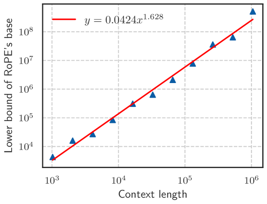
This image is a technical line-and-scatter plot on a log-log scale. It illustrates the relationship between the "Context length" of a model and the "Lower bound of RoPE's base." The chart includes a series of discrete data points and a fitted regression line with an associated mathematical formula.
## 2. Component Isolation
### A. Header / Legend Area
* **Location:** Top-left quadrant of the chart area.
* **Legend Item:** A solid red line segment followed by the mathematical expression: $y = 0.0424x^{1.628}$.
* **Visual Confirmation:** The red line in the legend matches the solid red trend line passing through the data points.
### B. Main Chart Area (Data Series)
* **Grid:** Light gray dashed grid lines for both major X and Y axes.
* **Data Points (Scatter):** Represented by dark blue triangles ($\black upward \text{ triangles}$).
* **Trend Line:** A solid red line.
* **Trend Verification:** The data points follow a consistent upward linear path on this log-log scale, indicating a power-law relationship. The red line acts as a "best fit" for these points.
### C. Axis Definitions
* **X-Axis (Horizontal):**
* **Label:** "Context length"
* **Scale:** Logarithmic (Base 10).
* **Markers:** $10^3, 10^4, 10^5, 10^6$.
* **Y-Axis (Vertical):**
* **Label:** "Lower bound of RoPE's base"
* **Scale:** Logarithmic (Base 10).
* **Markers:** $10^4, 10^5, 10^6, 10^7, 10^8$.
## 3. Data Extraction and Reconstructed Table
Based on the log-log scale, the following data points (blue triangles) are estimated from their spatial positioning relative to the grid:
| Context length (x) | Lower bound of RoPE's base (y) | Notes |
| :--- | :--- | :--- |
| $\approx 10^3$ | $\approx 4 \times 10^3$ | First data point |
| $\approx 2 \times 10^3$ | $\approx 1.5 \times 10^4$ | Slightly above the $10^4$ line |
| $\approx 4 \times 10^3$ | $\approx 3 \times 10^4$ | |
| $\approx 8 \times 10^3$ | $\approx 8 \times 10^4$ | Just below the $10^5$ line |
| $\approx 1.5 \times 10^4$ | $\approx 3 \times 10^5$ | |
| $\approx 3 \times 10^4$ | $\approx 6 \times 10^5$ | |
| $\approx 6 \times 10^4$ | $\approx 2 \times 10^6$ | |
| $\approx 1.2 \times 10^5$ | $\approx 8 \times 10^6$ | Just below the $10^7$ line |
| $\approx 2.5 \times 10^5$ | $\approx 4 \times 10^7$ | |
| $\approx 5 \times 10^5$ | $\approx 7 \times 10^7$ | |
| $\approx 10^6$ | $\approx 4 \times 10^8$ | Final data point |
## 4. Key Trends and Mathematical Findings
* **Relationship Type:** The data exhibits a strong power-law relationship, evidenced by the straight-line fit on a log-log plot.
* **Regression Formula:** The relationship is defined by the equation:
$$y = 0.0424x^{1.628}$$
* **Growth Rate:** The exponent of $1.628$ indicates that the lower bound of the RoPE (Rotary Positional Embedding) base grows super-linearly with respect to the context length. Specifically, as the context length increases by a factor of 10, the lower bound increases by a factor of approximately $10^{1.628} \approx 42.46$.
* **Observation:** The blue triangle data points show minor variance (noise) around the red regression line but maintain a very high correlation with the predicted model.