\n
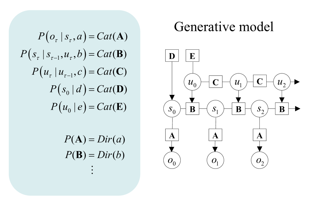
## Probabilistic Generative Model Diagram
### Overview
The image displays a technical diagram of a probabilistic generative model, split into two primary sections. On the left, within a light blue rounded rectangle, is a set of mathematical equations defining the model's probability distributions. On the right is a corresponding graphical model (a Bayesian network) titled "Generative model," which visually represents the dependencies between variables over discrete time steps. The diagram illustrates a sequential process involving observations, latent states, and control inputs.
### Components/Axes
The diagram is composed of two main components:
1. **Left Panel (Mathematical Definitions):** Contains a list of probability distributions.
2. **Right Panel (Graphical Model):** A directed acyclic graph showing variables as nodes and dependencies as arrows. The graph is organized into three horizontal layers over time steps (τ = 0, 1, 2,...).
**Graphical Model Node Types:**
* **Circular Nodes:** Represent random variables.
* `o_τ`: Observation at time τ.
* `s_τ`: Latent state at time τ.
* `u_τ`: Control input or action at time τ.
* **Square Nodes:** Represent fixed parameters or hyperparameters.
* `A`, `B`, `C`, `D`, `E`: Parameter matrices/vectors for the categorical distributions.
* `a`, `b`, `c`, `d`, `e`: Hyperparameters for the Dirichlet priors (implied by the equations).
**Graphical Model Flow & Connections:**
* **Vertical Flow (Generative Process):** Arrows point downward, indicating the direction of conditional dependence in the generative process.
* Parameters `D` and `E` influence the initial state `s_0` and initial input `u_0`, respectively.
* Parameters `C` connect consecutive control inputs (`u_τ-1` to `u_τ`).
* Parameters `B` connect consecutive states (`s_τ-1` to `s_τ`) and are also influenced by the current control input `u_τ`.
* Parameters `A` connect the current state `s_τ` to the observation `o_τ`.
* **Horizontal Flow (Time):** The model unfolds over time from left (τ=0) to right (τ=1, 2,...), indicated by the sequence of `u`, `s`, and `o` nodes and the right-pointing arrows from `u_2` and `s_2`.
### Detailed Analysis
**1. Mathematical Equations (Left Panel):**
The equations define a hierarchical Bayesian model with categorical observations and Dirichlet priors.
* `P(o_τ | s_τ, a) = Cat(A)`: The observation `o_τ` at time τ is drawn from a Categorical distribution parameterized by `A`, conditioned on the current state `s_τ` and some fixed parameter `a`.
* `P(s_τ | s_τ-1, u_τ, b) = Cat(B)`: The state `s_τ` transitions from the previous state `s_τ-1` and current input `u_τ` via a Categorical distribution parameterized by `B`, with hyperparameter `b`.
* `P(u_τ | u_τ-1, c) = Cat(C)`: The control input `u_τ` depends on the previous input `u_τ-1` through a Categorical distribution parameterized by `C`, with hyperparameter `c`.
* `P(s_0 | d) = Cat(D)`: The initial state `s_0` is drawn from a Categorical distribution parameterized by `D`, with hyperparameter `d`.
* `P(u_0 | e) = Cat(E)`: The initial control input `u_0` is drawn from a Categorical distribution parameterized by `E`, with hyperparameter `e`.
* `P(A) = Dir(a)`, `P(B) = Dir(b)`, `⋮`: The parameters `A`, `B`, etc., themselves have Dirichlet prior distributions with hyperparameters `a`, `b`, etc. The ellipsis (`⋮`) indicates this pattern continues for parameters `C`, `D`, and `E`.
**2. Graphical Model (Right Panel):**
The diagram visually instantiates the equations for the first three time steps (τ=0, 1, 2).
* **Initial Conditions (Top-Left):** Nodes `D` and `E` (squares) have arrows pointing to `s_0` and `u_0` (circles), respectively, representing the initial state and input distributions.
* **Time Step τ=0:** The initial state `s_0` and input `u_0` are connected via a `B` parameter node to generate the next state `s_1`. The state `s_0` also connects via an `A` parameter node to generate observation `o_0`.
* **Time Step τ=1:** The state `s_1` and input `u_1` (which depends on `u_0` via `C`) connect via `B` to generate `s_2`. The state `s_1` connects via `A` to generate observation `o_1`.
* **Time Step τ=2:** The pattern continues, with `s_2` and `u_2` leading to a subsequent state (implied by the right-pointing arrow from `s_2`), and `s_2` generating observation `o_2` via `A`.
* **Control Input Chain:** The `u` nodes (`u_0`, `u_1`, `u_2`) are connected horizontally by `C` parameter nodes, showing the autoregressive dependency of inputs.
### Key Observations
1. **Recursive Structure:** The model exhibits a clear recursive, state-space structure common in hidden Markov models (HMMs) and control systems. The state `s_τ` is a Markov blanket, summarizing the past to predict the future.
2. **Dual Dependency for States:** The state transition `P(s_τ | ...)` depends on both the previous state (`s_τ-1`) and the current control input (`u_τ`), making it a controlled Markov process.
3. **Separate Input Dynamics:** The control inputs `u_τ` have their own autoregressive dynamics (`P(u_τ | u_τ-1, c)`), modeled independently of the state.
4. **Parameter Sharing:** The same parameter nodes (`A`, `B`, `C`) are reused across all time steps, indicating parameter sharing and a stationary process (the rules don't change over time).
5. **Bayesian Hierarchy:** The model is fully Bayesian, with Dirichlet priors on the categorical parameters, allowing for uncertainty quantification and learning from data.
### Interpretation
This diagram defines a **controlled, autoregressive state-space model** with categorical variables. It is a generative recipe for creating sequences of observations (`o_0, o_1, o_2,...`) by first sampling initial conditions, then recursively sampling states and inputs.
* **What it represents:** This is a classic model for **sequential decision-making** or **robotics**. The `u` variables could be actions taken by an agent, the `s` variables are the hidden states of the environment, and the `o` variables are the agent's noisy perceptions. The model can be used for planning (generating action sequences) or learning (inferring states and parameters from observed data).
* **Relationships:** The core relationship is that the observable world (`o`) is generated from a hidden state (`s`), which itself evolves based on its own history and the agent's actions (`u`). The agent's actions also have their own momentum or policy (`C`).
* **Notable Anomaly/Feature:** The inclusion of explicit parameters `D` and `E` for the initial conditions is noteworthy. It formally separates the initialization process from the recursive dynamics, which is crucial for clear model specification.
* **Underlying Logic:** The use of Categorical distributions suggests the state, action, and observation spaces are discrete. The Dirichlet priors are conjugate to the Categorical likelihood, which simplifies mathematical inference (e.g., using Gibbs sampling). The ellipsis (`⋮`) implies the model is extensible to more parameters or time steps.
**In essence, this image provides a complete specification for a probabilistic program that can generate synthetic time-series data mimicking a controlled, discrete system, or conversely, be used to infer the hidden causes of real-world sequential data.**