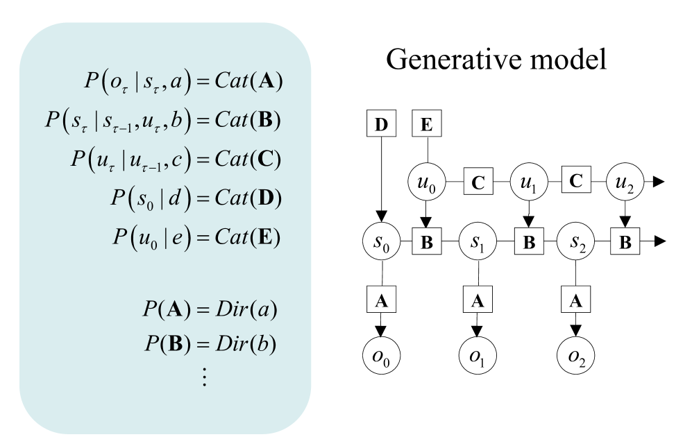
## Diagram: Generative Model
### Overview
The image presents a graphical representation of a generative model, likely used in a probabilistic or statistical context. It consists of two main parts: a set of probability equations on the left, enclosed in a rounded rectangle, and a directed acyclic graph (DAG) on the right, illustrating the relationships between different variables.
### Components/Axes
* **Title:** "Generative model" located at the top-right of the image.
* **Probability Equations (Left):**
* `P(o_τ | s_τ, a) = Cat(A)`
* `P(s_τ | s_{τ-1}, u_τ, b) = Cat(B)`
* `P(u_τ | u_{τ-1}, c) = Cat(C)`
* `P(s_0 | d) = Cat(D)`
* `P(u_0 | e) = Cat(E)`
* `P(A) = Dir(a)`
* `P(B) = Dir(b)`
* `...` (Indicates continuation of similar equations)
* **Directed Acyclic Graph (DAG) (Right):**
* Nodes: Represented by circles and squares, labeled with variables.
* Edges: Represented by arrows, indicating dependencies between variables.
* Variables: `D`, `E`, `u_0`, `u_1`, `u_2`, `s_0`, `s_1`, `s_2`, `o_0`, `o_1`, `o_2`.
* Factors: `A`, `B`, `C`
### Detailed Analysis
**Probability Equations:**
* The equations define conditional probabilities, where the probability of a variable depends on the values of other variables.
* `Cat(X)` likely represents a categorical distribution parameterized by `X`.
* `Dir(x)` likely represents a Dirichlet distribution parameterized by `x`.
* The subscript `τ` denotes a time step or index.
**Directed Acyclic Graph (DAG):**
* **Top Row:** `D` and `E` are at the top, with arrows pointing to `u_0` and `s_0` respectively.
* **Second Row:** `u_0`, `u_1`, and `u_2` are connected sequentially with edges labeled `C`.
* **Third Row:** `s_0`, `s_1`, and `s_2` are connected sequentially with edges labeled `B`. Each `u_i` also has a directed edge to the subsequent `s_i`.
* **Bottom Row:** `o_0`, `o_1`, and `o_2` are at the bottom.
* **Connections:** Each `s_i` has a directed edge to the corresponding `o_i`, labeled `A`.
* **Flow:** The graph suggests a temporal or sequential process, where the state `s` and observation `o` evolve over time, influenced by variables `u`, `D`, and `E`.
**Node and Factor Placement:**
* `D` is positioned above `s_0`, and has a directed edge to `s_0`.
* `E` is positioned above `u_0`, and has a directed edge to `u_0`.
* `C` is positioned between each `u_i` node.
* `B` is positioned between each `s_i` node.
* `A` is positioned between each `s_i` and `o_i` node.
### Key Observations
* The model appears to be a Hidden Markov Model (HMM) or a variant thereof, with hidden states `s` and observations `o`.
* The variables `u`, `D`, and `E` seem to influence the state transitions and initial states.
* The factors `A`, `B`, and `C` parameterize the conditional probabilities between the variables.
### Interpretation
The diagram represents a generative model that describes how a sequence of observations `o` is generated from a sequence of hidden states `s`. The model incorporates external influences `u`, `D`, and `E` that affect the state transitions and initial states. The probability equations on the left provide the mathematical formulation of the model, specifying the conditional probabilities between the variables. The DAG visually represents the dependencies between the variables, illustrating the flow of information and the generative process. This type of model is commonly used in various applications, such as speech recognition, natural language processing, and time series analysis.