## Diagram: Generative Model with Probabilistic Transitions
### Overview
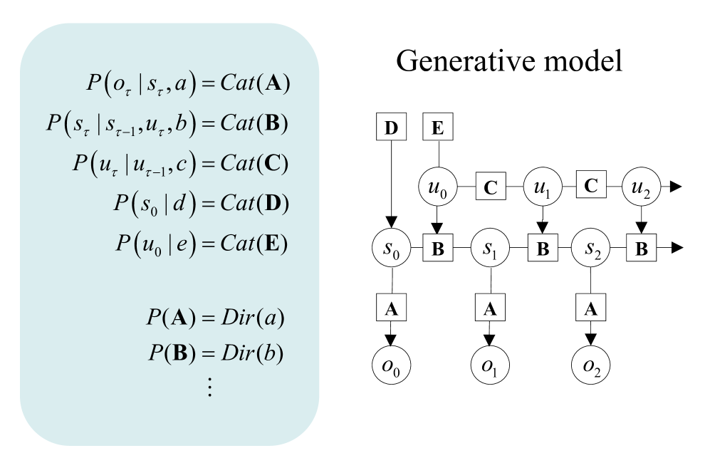
The image presents a hybrid representation of a probabilistic generative model, combining mathematical equations on the left with a state transition diagram on the right. The model appears to describe sequential decision-making processes with observable outputs and hidden states.
### Components/Axes
**Left Panel (Equations):**
- **Probability Definitions:**
- $ P(o_\tau | s_\tau, a) = \text{Cat}(A) $: Observation probability given state and action
- $ P(s_\tau | s_{\tau-1}, u_\tau, b) = \text{Cat}(B) $: State transition probability
- $ P(u_\tau | u_{\tau-1}, c) = \text{Cat}(C) $: Action selection probability
- $ P(s_0 | d) = \text{Cat}(D) $: Initial state distribution
- $ P(u_0 | e) = \text{Cat}(E) $: Initial action distribution
- **Dirichlet Priors:**
- $ P(A) = \text{Dir}(a) $
- $ P(B) = \text{Dir}(b) $
- ... (continuation implied)
**Right Panel (Diagram):**
- **Nodes:**
- **Inputs:** D, E (connected to initial state/action)
- **States:** $ s_0 \rightarrow s_1 \rightarrow s_2 $
- **Actions:** $ u_0 \rightarrow u_1 \rightarrow u_2 $
- **Observations:** $ o_0 \rightarrow o_1 \rightarrow o_2 $
- **Transitions:**
- Solid arrows between states (B transitions)
- Dashed arrows from states to observations (A transitions)
- Input nodes D/E connected to initial state/action via arrows
### Detailed Analysis
**Mathematical Structure:**
1. **Observation Model:** $ P(o_\tau | s_\tau, a) $ suggests observations depend on current state and action
2. **State Dynamics:** $ P(s_\tau | s_{\tau-1}, u_\tau, b) $ indicates Markovian state transitions influenced by actions
3. **Action Selection:** $ P(u_\tau | u_{\tau-1}, c) $ implies action persistence/change over time
4. **Initial Conditions:** $ P(s_0 | d) $ and $ P(u_0 | e) $ define starting distributions
**Diagram Flow:**
- Inputs D → Initial state $ s_0 $
- Input E → Initial action $ u_0 $
- State transitions: $ s_0 \xrightarrow{B} s_1 \xrightarrow{B} s_2 $
- Action transitions: $ u_0 \xrightarrow{C} u_1 \xrightarrow{C} u_2 $
- Observation emissions: Each state emits observation via $ P(o_\tau | s_\tau, a) = \text{Cat}(A) $
### Key Observations
1. **Markovian Structure:** The model assumes Markov properties for both state transitions and action selection
2. **Categorical Distributions:** All probability distributions are categorical (Cat), suggesting discrete state/action spaces
3. **Hierarchical Priors:** Dirichlet distributions provide conjugate priors for the categorical parameters
4. **Temporal Coupling:** Actions persist across time steps ($ u_\tau $ depends on $ u_{\tau-1} $)
### Interpretation
This appears to be a **Partially Observable Markov Decision Process (POMDP)** framework with:
- **Hidden States:** $ s_\tau $ (only partially observable through $ o_\tau $)
- **Temporal Dependencies:** Both state transitions and action selection exhibit temporal correlation
- **Bayesian Inference:** The use of Dirichlet priors suggests a Bayesian approach to parameter estimation
- **Sequential Decision Making:** The model captures the interplay between observations, hidden states, and actions over time
The diagram visually reinforces the equations by showing:
1. Input nodes D/E seeding initial conditions
2. Sequential state transitions governed by parameter B
3. Action persistence through parameter C
4. Observation generation through parameter A
5. The cyclical nature of perception-action loops in sequential decision-making systems