## Directed Acyclic Graph (DAG): Hierarchical Variable Dependencies
### Overview
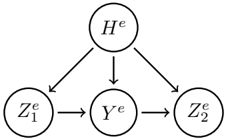
The image displays a directed acyclic graph (DAG), a type of diagram commonly used in statistics, machine learning, and causal inference to represent dependencies between variables. The graph consists of five nodes (circles) connected by directed edges (arrows), illustrating a specific flow of influence or conditional dependence.
### Components
* **Nodes (Variables):** There are five nodes, each containing a mathematical symbol.
* **Top Node:** `H^e` (H with a superscript "e").
* **Bottom Row Nodes (Left to Right):**
* `Z_1^e` (Z with subscript "1" and superscript "e").
* `Y^e` (Y with a superscript "e").
* `Z_2^e` (Z with subscript "2" and superscript "e").
* **Edges (Relationships):** The arrows indicate directed relationships.
* Three arrows originate from `H^e`, pointing downward to `Z_1^e`, `Y^e`, and `Z_2^e` respectively.
* One arrow points horizontally from `Z_1^e` to `Y^e`.
* One arrow points horizontally from `Y^e` to `Z_2^e`.
### Detailed Analysis
The graph defines a precise structure of dependencies:
1. **Common Parent:** The variable `H^e` is a common parent or source node. It has a direct influence on all three variables in the lower tier (`Z_1^e`, `Y^e`, and `Z_2^e`).
2. **Sequential Chain:** Among the lower-tier variables, there is a sequential, left-to-right dependency chain: `Z_1^e` influences `Y^e`, which in turn influences `Z_2^e`.
3. **Spatial Layout:** `H^e` is positioned centrally at the top. The three dependent variables are arranged in a horizontal line below it, with `Z_1^e` on the left, `Y^e` in the center, and `Z_2^e` on the right. The arrows from `H^e` fan out to each of them.
### Key Observations
* The superscript `e` is consistently applied to all variables (`H^e`, `Z_1^e`, `Y^e`, `Z_2^e`), suggesting they belong to the same model, experiment, or context (e.g., "estimated," "experimental," or a specific entity `e`).
* The graph contains no cycles; all paths follow the direction of the arrows without looping back.
* `Y^e` is a mediator. It is directly influenced by both `H^e` and `Z_1^e`, and it directly influences `Z_2^e`.
* `Z_1^e` and `Z_2^e` are not directly connected; their relationship is mediated through `Y^e`.
### Interpretation
This diagram represents a **conditional dependency structure**. It suggests a data-generating process or a causal model where:
* `H^e` is a high-level or latent variable that affects all observed or lower-level variables.
* There is a temporal or causal sequence among the lower variables: `Z_1^e` occurs first, affecting `Y^e`, which then affects `Z_2^e`.
* The model implies that to understand the relationship between `Z_1^e` and `Z_2^e`, one must account for the mediating variable `Y^e` and the confounding or common-cause variable `H^e`.
**Example Context:** This structure is common in:
* **Structural Equation Modeling (SEM):** Where `H^e` could be a hidden construct, `Z_1^e` and `Z_2^e` are indicators, and `Y^e` is an intermediate outcome.
* **Time Series or Sequential Models:** Where `H^e` is a global parameter, and `Z_1^e`, `Y^e`, `Z_2^e` are states at consecutive time steps.
* **Causal Inference:** Where `H^e` is a pre-treatment covariate, `Z_1^e` is an initial treatment or exposure, `Y^e` is an intermediate outcome, and `Z_2^e` is a final outcome.
The graph provides a clear, falsifiable hypothesis about how these five variables relate to one another, guiding analysis on which dependencies to estimate and which conditional independencies to test.