## Density Histogram: Twenty-first Day (July 31, 1872)
### Overview
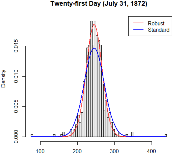
The image is a histogram showing the density distribution of some variable on the twenty-first day, July 31, 1872. Two curves are overlaid on the histogram: a "Robust" fit (red) and a "Standard" fit (blue). The histogram bars are black and white.
### Components/Axes
* **Title:** Twenty-first Day (July 31, 1872)
* **X-axis:** Values ranging from 100 to 400, with markers at 100, 200, 300, and 400.
* **Y-axis:** Density, ranging from 0.000 to 0.015, with markers at 0.000, 0.005, 0.010, and 0.015.
* **Legend:** Located in the top-right corner.
* **Robust:** Red line
* **Standard:** Blue line
### Detailed Analysis
* **Histogram:** The histogram shows a distribution centered around 250. The frequency of values decreases as you move away from the center in either direction.
* **Robust (Red) Curve:** This curve is more peaked and narrower than the "Standard" curve. It appears to fit the central portion of the histogram more closely. The peak of the red curve is approximately at a density of 0.017, centered around x=250.
* **Standard (Blue) Curve:** This curve is broader and flatter than the "Robust" curve. It appears to capture the overall shape of the distribution, including the tails. The peak of the blue curve is approximately at a density of 0.013, centered around x=250.
* **X-Axis Values:**
* 100
* 200
* 300
* 400
* **Y-Axis Values:**
* 0.000
* 0.005
* 0.010
* 0.015
### Key Observations
* Both curves are centered around the same x-value (approximately 250).
* The "Robust" curve has a higher peak and narrower spread than the "Standard" curve.
* The histogram shows some data points outside the range well-captured by either curve, particularly in the tails.
### Interpretation
The graph compares two different statistical models ("Robust" and "Standard") fitted to the same data. The "Robust" model seems to be less sensitive to outliers, resulting in a narrower distribution that focuses on the central tendency of the data. The "Standard" model is more influenced by outliers, leading to a broader distribution. The choice between the two models depends on the specific application and the importance of accounting for outliers. The data appears to be unimodal and approximately normally distributed, although there are some deviations from normality, especially in the tails.