## Histogram with Overlaid Density Curves: Twenty-first Day (July 31, 1872)
### Overview
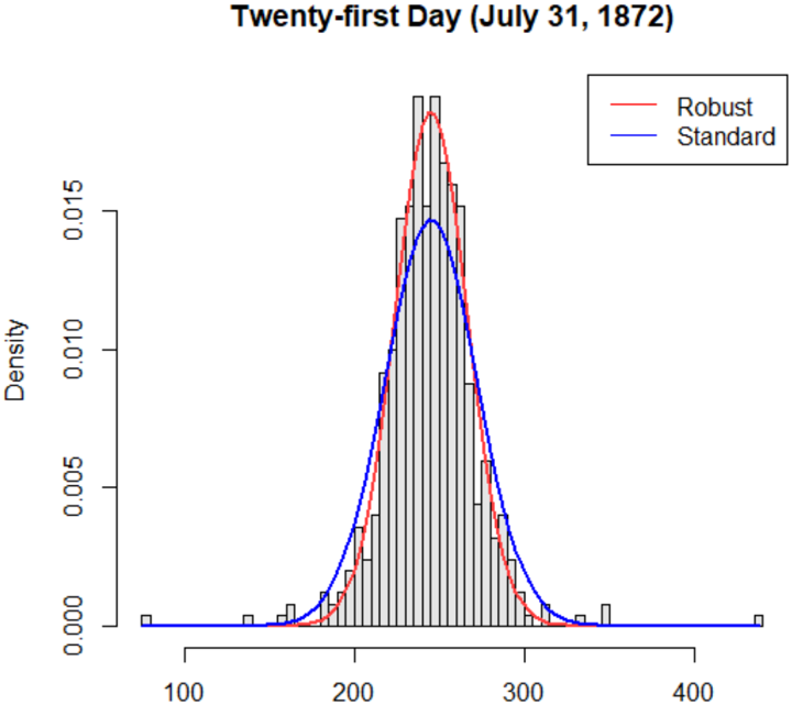
The image is a statistical chart displaying a histogram of data with two overlaid probability density function curves. The chart is titled "Twenty-first Day (July 31, 1872)". It compares two different methods of estimating the data's distribution, labeled "Robust" and "Standard".
### Components/Axes
* **Title:** "Twenty-first Day (July 31, 1872)" - centered at the top.
* **Y-Axis:** Labeled "Density". The scale runs from 0.000 to approximately 0.018, with major tick marks at 0.000, 0.005, 0.010, and 0.015.
* **X-Axis:** Unlabeled, but represents a numerical variable. The scale runs from approximately 80 to 440, with major tick marks and labels at 100, 200, 300, and 400.
* **Legend:** Located in the top-right corner, inside a box. It contains two entries:
* A red line labeled "Robust".
* A blue line labeled "Standard".
* **Histogram:** A series of vertical, light gray bars with black outlines. The bars represent the frequency distribution of the underlying dataset.
* **Density Curves:**
* **Red Curve ("Robust"):** A smooth, continuous line overlaid on the histogram.
* **Blue Curve ("Standard"):** A smooth, continuous line overlaid on the histogram.
### Detailed Analysis
* **Histogram Distribution:** The data is unimodal and roughly symmetric, centered around a value of approximately 250. The distribution has a moderate spread, with most data falling between 200 and 300. There are a few sparse data points (very short bars) extending to the left towards 100 and to the right towards 400.
* **"Robust" Density Curve (Red):**
* **Trend:** This curve has a sharp, narrow peak. It rises steeply from near zero around x=180, peaks sharply, and falls steeply back to near zero around x=320.
* **Peak:** The peak is the highest point on the entire chart, reaching a density value of approximately **0.017** at an x-value of about **250**.
* **Width:** The curve is notably narrower than the blue curve, indicating a lower estimated variance or a method less influenced by potential outliers.
* **"Standard" Density Curve (Blue):**
* **Trend:** This curve has a broader, more rounded peak. It rises more gradually from near zero around x=150, peaks, and descends more gradually, returning to near zero around x=350.
* **Peak:** The peak is lower than the red curve's peak, reaching a density value of approximately **0.014** at an x-value of about **250**.
* **Width:** The curve is wider, suggesting a higher estimated variance or a standard method that gives more weight to the tails of the distribution.
### Key Observations
1. **Peak Discrepancy:** The "Robust" method estimates a significantly higher peak density (~0.017) compared to the "Standard" method (~0.014) at the same central location (x≈250).
2. **Width Discrepancy:** The "Robust" curve is narrower, while the "Standard" curve is wider. This is the most visually striking difference.
3. **Central Alignment:** Both density curves and the histogram's mode are aligned at approximately x=250, confirming this as the central tendency of the data.
4. **Histogram Fit:** The histogram bars appear to be more closely followed by the taller, narrower "Robust" curve near the peak, while the "Standard" curve seems to smooth over the peak more.
### Interpretation
This chart visually demonstrates the difference between two statistical estimation techniques applied to the same dataset from July 31, 1872.
* **What it suggests:** The "Robust" method produces an estimate that is more concentrated around the central value (250), implying it is less sensitive to data points in the tails (the sparse bars near 100 and 400). The "Standard" method produces a more dispersed estimate, which could be the result of a technique (like a standard kernel density estimate) that is more influenced by all data points equally, including potential outliers.
* **Relationship between elements:** The histogram provides the raw data context. The two curves are competing models of the data's underlying probability distribution. Their contrasting shapes highlight how methodological choices can lead to different interpretations of the same data's spread and concentration.
* **Notable implication:** The choice between a "Robust" and "Standard" method matters significantly for this dataset. If the goal is to identify the most typical or frequent value, the Robust estimate suggests a stronger concentration. If the goal is to account for all observed variability, including extremes, the Standard estimate provides a broader picture. The chart itself does not indicate which method is "correct," but it effectively illustrates their divergent conclusions.