# Technical Document Extraction: Multi-Layer Perceptron (MLP) vs. Kolmogorov-Arnold Network (KAN)
## Table Structure
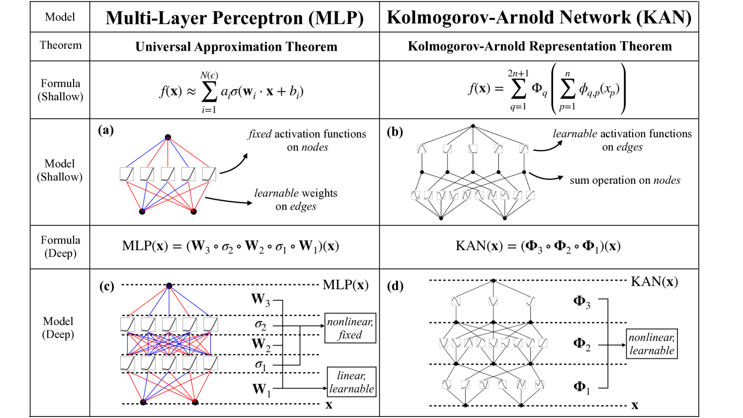
| Model | Multi-Layer Perceptron (MLP) | Kolmogorov-Arnold Network (KAN) |
|-------|------------------------------|----------------------------------|
| Theorem | Universal Approximation Theorem | Kolmogorov-Arnold Representation Theorem |
| Formula (Shallow) | \( f(\mathbf{x}) \approx \sum_{i=1}^{N(\epsilon)} a_i\sigma(\mathbf{w}_i \cdot \mathbf{x} + b_i) \) | \( f(\mathbf{x}) = \sum_{q=1}^{2n+1} \Phi_q\left(\sum_{p=1}^n \phi_{q,p}(x_p)\right) \) |
| Model (Shallow) | Diagram (a) | Diagram (b) |
| Formula (Deep) | \( \text{MLP}(\mathbf{x}) = (\mathbf{W}_3 \circ \sigma_2 \circ \mathbf{W}_2 \circ \sigma_1 \circ \mathbf{W}_1)(\mathbf{x}) \) | \( \text{KAN}(\mathbf{x}) = (\Phi_3 \circ \Phi_2 \circ \Phi_1)(\mathbf{x}) \) |
| Model (Deep) | Diagram (c) | Diagram (d) |
---
## Key Components and Flow
### 1. **Model (Shallow)**
#### (a) Multi-Layer Perceptron (MLP)
- **Fixed Activation Functions**: Applied to nodes (σ).
- **Learnable Weights**: Applied to edges (w, b).
- **Diagram (a)**:
- Nodes represented as squares with σ symbols.
- Edges with red (weights) and blue (bias) lines.
- Output node aggregates inputs via summation.
#### (b) Kolmogorov-Arnold Network (KAN)
- **Learnable Activation Functions**: Applied to edges (Φ).
- **Sum Operation**: Applied to nodes.
- **Diagram (b)**:
- Nodes represented as circles with Φ symbols.
- Edges with black lines.
- Output node aggregates inputs via summation.
---
### 2. **Model (Deep)**
#### (c) Multi-Layer Perceptron (MLP)
- **Layers**:
- **Input Layer**: Linear, learnable weights (W₁).
- **Hidden Layers**: Nonlinear, fixed activation (σ₁, σ₂).
- **Output Layer**: Nonlinear, fixed activation (σ).
- **Diagram (c)**:
- Three layers (W₁, W₂, W₃) with σ₁, σ₂, σ.
- Red lines for weights, blue for bias, black for activation functions.
#### (d) Kolmogorov-Arnold Network (KAN)
- **Layers**:
- **Input Layer**: Linear, learnable weights (Φ₁).
- **Hidden Layers**: Nonlinear, learnable activation (Φ₂, Φ₃).
- **Diagram (d)**:
- Three layers (Φ₁, Φ₂, Φ₃) with Φ symbols.
- Black lines for edges, Φ symbols for activation functions.
---
## Mathematical Formulas
### MLP (Shallow)
\[ f(\mathbf{x}) \approx \sum_{i=1}^{N(\epsilon)} a_i\sigma(\mathbf{w}_i \cdot \mathbf{x} + b_i) \]
- **σ**: Fixed sigmoid activation.
- **w, b**: Learnable weights and biases.
### KAN (Shallow)
\[ f(\mathbf{x}) = \sum_{q=1}^{2n+1} \Phi_q\left(\sum_{p=1}^n \phi_{q,p}(x_p)\right) \]
- **Φ**: Learnable activation functions.
- **φ**: Input-dependent functions.
### MLP (Deep)
\[ \text{MLP}(\mathbf{x}) = (\mathbf{W}_3 \circ \sigma_2 \circ \mathbf{W}_2 \circ \sigma_1 \circ \mathbf{W}_1)(\mathbf{x}) \]
- **σ₁, σ₂, σ**: Fixed nonlinear activations.
- **W₁, W₂, W₃**: Learnable weight matrices.
### KAN (Deep)
\[ \text{KAN}(\mathbf{x}) = (\Phi_3 \circ \Phi_2 \circ \Phi_1)(\mathbf{x}) \]
- **Φ₁, Φ₂, Φ₃**: Learnable nonlinear activations.
---
## Diagram Analysis
### Spatial Grounding
- **Legend**: Not explicitly present; inferred from diagram annotations.
- **Color Coding**:
- **Red**: Learnable weights (MLP) / Non-learnable weights (KAN).
- **Blue**: Bias terms (MLP).
- **Black**: Activation functions (MLP) / Learnable activations (KAN).
### Trend Verification
- **MLP (Shallow)**: Linear combination of fixed sigmoid activations.
- **KAN (Shallow)**: Sum of learnable activation functions.
- **MLP (Deep)**: Sequential composition of linear and fixed nonlinear layers.
- **KAN (Deep)**: Sequential composition of learnable nonlinear functions.
---
## Critical Observations
1. **Activation Flexibility**:
- MLP: Fixed activations (σ) on nodes.
- KAN: Learnable activations (Φ) on edges.
2. **Operations**:
- MLP: Summation at nodes.
- KAN: Summation at nodes with learnable Φ functions.
3. **Scalability**:
- MLP: Depth increases via stacked linear+nonlinear layers.
- KAN: Depth increases via chained learnable Φ functions.
---
## Language Notes
- **Primary Language**: English.
- **No Non-English Text Detected**.