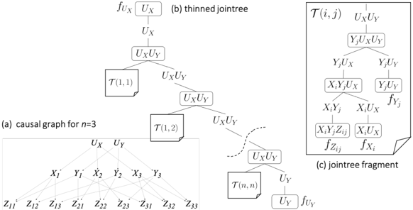
## Diagram: Causal Graph and Jointree Representation for n=3 ### Overview The image is a technical diagram from the field of probabilistic graphical models or causal inference. It illustrates three interconnected representations: (a) a causal graph for a system with three units (n=3), (b) a corresponding "thinned jointree" derived from the graph, and (c) a detailed fragment of a cluster within that jointree. The diagram demonstrates the structural relationship between a causal model and its factorization into a junction tree for efficient computation. ### Components/Axes The diagram is divided into three labeled parts: **Part (a): Causal Graph for n=3** * **Title:** "(a) causal graph for n=3" * **Nodes (Variables):** * Top Layer: `U_X`, `U_Y` (Latent or exogenous variables) * Middle Layer: `X_1`, `Y_1`, `X_2`, `Y_2`, `X_3`, `Y_3` (Observed variables for units 1, 2, 3) * Bottom Layer: `Z_11`, `Z_12`, `Z_13`, `Z_21`, `Z_22`, `Z_23`, `Z_31`, `Z_32`, `Z_33` (Observed variables, likely outcomes or measurements) * **Edges (Dependencies):** Directed arrows show the flow of influence: * `U_X` points to all `X_i` nodes. * `U_Y` points to all `Y_i` nodes. * Each `X_i` and `Y_i` pair points to the corresponding set of `Z_ij` nodes for that unit `i`. For example, `X_1` and `Y_1` both point to `Z_11`, `Z_12`, and `Z_13`. **Part (b): Thinned Jointree** * **Title:** "(b) thinned jointree" * **Structure:** A tree (acyclic graph) of clusters (nodes) connected by separators (edges). * **Clusters (Nodes):** Rectangular boxes containing sets of variables. * Root Cluster: `U_X` * Child of Root: `U_X U_Y` * Subsequent Clusters: `T(1,1)`, `U_X U_Y`, `T(1,2)`, `U_X U_Y`, ... leading to `T(n,n)`, `U_Y`. * Leaf Cluster: `U_Y` * **Separators (Edge Labels):** The variable sets on the edges between clusters. * Edge from `U_X` to `U_X U_Y`: Label `U_X` * Edge from `U_X U_Y` to `T(1,1)`: Label `U_X U_Y` * Edge from `U_X U_Y` to next `U_X U_Y`: Label `U_X U_Y` * (Pattern continues, with `U_X U_Y` being the common separator between many clusters). * Final edge into leaf `U_Y`: Label `U_Y` * **Functions:** Notations `f_{U_X}` and `f_{U_Y}` are placed near the root (`U_X`) and leaf (`U_Y`) clusters, respectively, indicating potential functions associated with those variables. **Part (c): Jointree Fragment** * **Title:** "(c) jointree fragment" * **Content:** A detailed view of the internal structure of one of the `T(i,j)` clusters from the thinned jointree. * **Structure:** A small subtree or factor graph fragment. * **Nodes and Labels (from top to bottom):** * Top Node: `U_X U_Y` * Separator: `Y_j U_X U_Y` * Node: `Y_j U_X U_Y` * Separators: `Y_j U_X` (left), `Y_j U_Y` (right) * Left Node: `X_i Y_j U_X` * Right Node: `Y_j U_Y` * Separators from Left Node: `X_i Y_j` (left), `X_i U_X` (right) * Bottom-Left Node: `X_i Y_j Z_{ij}` * Bottom-Right Node: `X_i U_X` * **Functions:** Notations `f_{Z_{ij}}` and `f_{X_i}` are placed near the `X_i Y_j Z_{ij}` and `X_i U_X` nodes, respectively. ### Detailed Analysis 1. **Causal Graph (a):** This is a bipartite-like structure with two latent parents (`U_X`, `U_Y`) influencing all observed units. Each unit `i` has paired variables `X_i` and `Y_i`, which in turn generate multiple observations `Z_{ij}` (where `j` likely indexes different measurements or contexts for unit `i`). The graph implies that all `X` variables share a common cause `U_X`, and all `Y` variables share a common cause `U_Y`. 2. **Thinned Jointree (b):** This tree organizes the variables from the causal graph into clusters to enable efficient probabilistic inference. The "thinned" aspect suggests a simplification where many clusters contain only the global variables `U_X` and `U_Y`. The clusters labeled `T(i,j)` represent localized computations for specific unit pairs `(i,j)`. The tree flows from the global `U_X` cluster, through a series of `U_X U_Y` and `T(i,j)` clusters, to the global `U_Y` cluster. 3. **Jointree Fragment (c):** This zooms into a `T(i,j)` cluster, revealing it is not a simple node but contains a structured factorization. It shows how the joint probability for variables involving unit `i` and unit `j` (`X_i`, `Y_j`, `Z_{ij}`) and the global variables (`U_X`, `U_Y`) can be broken down. The functions `f_{Z_{ij}}` and `f_{X_i}` suggest local conditional probability distributions or factors. ### Key Observations * **Structural Consistency:** The variable sets in the separators of the thinned jointree (e.g., `U_X U_Y`) correctly reflect the intersections of the clusters they connect, adhering to the running intersection property of junction trees. * **Scalability Notation:** The use of `T(n,n)` and the ellipsis (`...`) in part (b) indicates the pattern generalizes for any number of units `n`, with the diagram specifically illustrating the case for `n=3`. * **Functional Annotation:** The placement of `f` functions (`f_{U_X}`, `f_{U_Y}`, `f_{Z_{ij}}`, `f_{X_i}`) at specific clusters indicates where in the tree structure the original factors from the probabilistic model are absorbed. * **Spatial Layout:** Part (a) is positioned at the bottom-left. Part (b) occupies the central and upper-right space, flowing diagonally from top-left to bottom-right. Part (c) is a detailed inset in the upper-right corner, connected by a dashed line to one of the `T(i,j)` clusters in part (b), explicitly showing it is a magnified view. ### Interpretation This diagram serves as a pedagogical or technical illustration of how to convert a specific type of causal model—a model with global latent variables (`U_X`, `U_Y`) influencing unit-level variables (`X_i`, `Y_i`), which in turn generate observations (`Z_{ij}`)—into a computational architecture (a thinned jointree) suitable for exact inference. The **key insight** is that the complex dependencies in the causal graph (a) can be managed by a jointree where most clusters are simple, containing only the global variables. The computationally intensive work is localized within the `T(i,j)` fragments (c), which handle the interactions between the global variables and the variables for specific units. This structure suggests an efficient algorithm where messages are passed primarily through the simple `U_X U_Y` clusters, with more complex computations isolated to the `T(i,j)` sub-structures. The diagram effectively bridges conceptual modeling (the causal graph) with practical implementation (the junction tree algorithm), showing how to structure computations to leverage the conditional independencies present in the original model. The "thinned" nature of the tree likely results from exploiting symmetries or independencies given the specific structure of the causal graph.